MIT | 数据分析、信号处理和机器学习中的矩阵方法 笔记系列 Lecture 6 Singular Value Decomposition (SVD)

本系列为MIT Gilbert Strang教授的"数据分析、信号处理和机器学习中的矩阵方法"的学习笔记。

• Gilbert Strang & Sarah Hansen | Sprint 2018
• 18.065: Matrix Methods in Data Analysis, Signal Processing, and Machine Learning
• 视频网址: https://ocw.mit.edu/courses/18-065-matrix-methods-in-data-analysis-signal-processing-and-machine-learning-spring-2018/
• 关注 下面的公众号，回复“ 矩阵方法 ”，即可获取 本系列完整的pdf笔记文件~

---

内容在CSDN、知乎和微信公众号同步更新

• CSDN博客
• 知乎
• 微信公众号
• qq邮箱: 981591477

• Markdown源文件暂未开源，如有需要可联系邮箱
• 笔记难免存在问题，欢迎联系邮箱指正

---

Lecture 0: Course Introduction

Lecture 1 The Column Space of $A$ Contains All Vectors $Ax$

Lecture 2 Multiplying and Factoring Matrices

Lecture 3 Orthonormal Columns in $Q$ Give $Q^{\prime }Q=I$

Lecture 4 Eigenvalues and Eigenvectors

Lecture 5 Positive Definite and Semidefinite Matrices

Lecture 6 Singular Value Decomposition (SVD)

Lecture 7 Eckart-Young: The Closest Rank $k$ Matrix to $A$

Lecture 8 Norms of Vectors and Matrices

Lecture 9 Four Ways to Solve Least Squares Problems

Lecture 10 Survey of Difficulties with $Ax=b$

Lecture 11 Minimizing ||x|| Subject to $Ax=b$

Lecture 12 Computing Eigenvalues and Singular Values

Lecture 13 Randomized Matrix Multiplication

Lecture 14 Low Rank Changes in $A$ and Its Inverse

Lecture 15 Matrices $A(t)$ Depending on $t$, Derivative = $dA/dt$

Lecture 16 Derivatives of Inverse and Singular Values

Lecture 17 Rapidly Decreasing Singular Values

Lecture 18 Counting Parameters in SVD, LU, QR, Saddle Points

Lecture 19 Saddle Points Continued, Maxmin Principle

Lecture 20 Definitions and Inequalities

Lecture 21 Minimizing a Function Step by Step

Lecture 22 Gradient Descent: Downhill to a Minimum

Lecture 23 Accelerating Gradient Descent (Use Momentum)

Lecture 24 Linear Programming and Two-Person Games

Lecture 25 Stochastic Gradient Descent

Lecture 26 Structure of Neural Nets for Deep Learning

Lecture 27 Backpropagation: Find Partial Derivatives

Lecture 28 Computing in Class [No video available]

Lecture 29 Computing in Class (cont.) [No video available]

Lecture 30 Completing a Rank-One Matrix, Circulants!

Lecture 31 Eigenvectors of Circulant Matrices: Fourier Matrix

Lecture 32 ImageNet is a Convolutional Neural Network (CNN), The Convolution Rule

Lecture 33 Neural Nets and the Learning Function

Lecture 34 Distance Matrices, Procrustes Problem

Lecture 35 Finding Clusters in Graphs

Lecture 36 Alan Edelman and Julia Language

---

---

Lecture 6 Singular Value Decomposition (SVD)

6.1 SVD的概念

• 奇异值 (Singular Values) VS 特征值 (Eigenvalues)

  • Singular Values 与 Eigenvalues 非常相似

  • 但 A 的 Singular Values 适用于rectangular matrices! 且有两个 singular vectors

  • 特征值、特征向量概念的局限：

    ❌ 仅适用于方阵：If A is Ax rectangular $\Rightarrow$ $\ne \lambda x$ $(m\times n\times n\times 1)=(m\times 1)$

    ❌ 即便A is square, 若A只是一个general而不是symmetric matrix $\Rightarrow$ A可能会有complex eigenvalues, not orthogonal eigenvectors, etc.

    🚩 $\Rightarrow$ 特征值、特征向量存在局限，需要新的概念 $\Rightarrow$ Singular Values

• 奇异值分解的概念

  • Compare with $S=Q\Lambda Q^T$

    ▪ $Q$: Eigenvectors (仅一个)

    ▪ $\Lambda$: Eigenvalues

  • now $A=U\Sigma V^T$

    ▪ $U$: Left Singular vectors in m dimensions

    ▪ $V^T$: Right Singular vectors in n dimensions

    ▪ $\Sigma$: Singular values

    ✅ $S=\left[\begin{array}{ccccc}{\sigma }_1& & & & \\ & {\sigma }_2& & & \\ & & ...& & \\ & & & {\sigma }_r& ...\end{array}\right]\in M\times N$

6.2 What are $U,V^T$ and $\Sigma$ in $A=U\Sigma V^T$?

• The key: $A^{T}A$ is a great matrix

  • $A$: $M\times N$

  • $A^T$: $N\times M$

  • $A^{T}A$: $N\times N$

  • and symmetric!!!

  • And: positive definite!

    ▪ All eigenvalues are > 0

• Therefore, $\exists V$, s.t.

  • $A^{T}A$ = $V\Lambda V^T$

    ▪ $V$: eigenvectors of $A^{T}A$ $\Rightarrow$ Orthogonal

    ▪ $\Lambda$: the eigenvalues of $\Lambda$ $\Rightarrow$ $\ge 0$

  • Note: $A{A}^T$ is a different guy! $\Rightarrow$ $A{A}^T=U\Lambda U^T$

  • Looking for: $A{v}_1={\sigma }_1{u}_1$ ( $AV=U\Sigma$的第1列 ), $A{v}_2={\sigma }_2{u}_2$ ( $AV=U\Sigma$的第2列 ), …, $A{v}_r={\sigma }_r{u}_r$ ( $AV=U\Sigma$的第r列 )

    🚩 Why stop at r (the rank)? 因为大于r时${\sigma }_r=0$

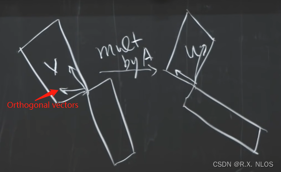
    🚩 $v_i$: a bunch of orthogonal vectors v;

    🚩 $u_i$: a bunch of orthogonal vectors u;

    🚩 这样，即可$A[v_1,v_2,...,v_r]=[u_1,u_2,...,u_r]\left[\begin{array}{ccccc}{\sigma }_1& & & & \\ & {\sigma }_2& & & \\ & & ...& & \\ & & & {\sigma }_r& ...\end{array}\right]$ $\Rightarrow$ $AV=U\Sigma \Rightarrow A=U\Sigma V^T$ (上述过程从vector-wise form变为了matrix form)

    🚩 几何表示如下图

• How to find the $V$, $U$, $\Sigma$ above?

  • 若$A=U\Sigma V^T$ $\Rightarrow$ $A^{T}A=V{\Sigma }^T{U}^{T}U\Sigma V^T$ = $V{\Sigma }^T\Sigma V^T$

  • 其中，已知 $A^{T}A$ 是 positive definite matrix

  • Therefore: 如下取值满足上式

    ✅ V: the eigenvectors of $A^{T}A$

    ✅ $({\Sigma }^T\Sigma )$: the eigenvalues of ${\Sigma }^T\Sigma$ $\Rightarrow$ ${\Sigma }^T\Sigma$ = [${\sigma }^2$] $\Rightarrow$ ${\sigma }^2$: eigenvalues of $A^{T}A$

  • 另一方面：$A{A}^T$ = $U\Sigma V^{T}V{\Sigma }^T{U}^T$ = $U(\Sigma {\Sigma }^T)U^T$ $\Rightarrow$

    ✅ U: the eigenvectors of $A{A}^T$

  • 最后一步：Given $A$ $\Rightarrow$ we can get $V$ (and $v_i$) and $\sigma$ $\Rightarrow$ $u_i$ should be $u_i=\frac{A{v}_i}{{\sigma }_r}$

    🚩 为什么根据$A{A}^T$得到的$U$ 就是 $u_i=\frac{A{v}_i}{{\sigma }_r}$

    🚩 即，已知$V$和$\Sigma$满足$A^{T}A=V{\Sigma }^T\Sigma V^T$ , 求证 $A=U\Sigma V^T$, 即 证明$U$ orthogonal , 即 证明$u_i^T{u}_j=0$ $(i\ne j)$

    👉 毕竟，若考虑到$A{A}^T$有多重根的情况，特征向量$u_i$可以有无数个

    🚩 $(\frac{A{v}_i}{{\sigma }_i}{)}^T(\frac{A{v}_j}{{\sigma }_j})$ $\Rightarrow$ 因为v are orthogonal vectors (eigenvectors of $A^{T}A$) $\Rightarrow$ $(\frac{A{v}_i}{{\sigma }_i}{)}^T(\frac{A{v}_j}{{\sigma }_j})=\frac{v_i^T{A}^{T}A{v}_j}{{\sigma }_i{\sigma }_j}=v_i^T{\sigma }_j^2{v}_j/({\sigma }_1{\sigma }_2)$ = 0.

    🚩 因此，$A^{T}A=V{\Sigma }^T\Sigma V^T$ $\Rightarrow$ $A^{T}A=V{\Sigma }^T{U}^{T}U\Sigma V^T$ $\Rightarrow$ $A=U\Sigma V^T$

  • 即，$V$, $AV$, $U$, $U\Sigma$ 都是orthogonal的

• SVD的计算

  • 证明过程中的计算方法: $A$ $\Rightarrow$ $A^{T}A$ $\Rightarrow$ $V,\Sigma$ $\Rightarrow$ $u=Av/\sigma$

    ❌ 缺点：$A^{T}A$ too large, too expensive ; Its vulnerability to round off errors (condition numver) is squared

6.3 Eigenvalues的意义

• SVD的 geometry meaning

  • $A=U\Sigma V$

  • $U$ and $V$: orthogonal $\Rightarrow$ rotation (也可能是reflection但not important)

  • $\Sigma$: diagonal $\Rightarrow$ stretching

  • For $Ax=U\Sigma V^{T}x$, geometry meaning 如下图

    ▪ assume ${\sigma }_1\ge {\sigma }_2\ge {\sigma }_3\ge ...$

    ▪ Every linear transformation can be factored into a rotation + a stretch + a different roration

    ▪ 什么时候两个rotation相等？$A=Q\Lambda Q^T$ 且 $\Lambda >0$ $\Rightarrow$ $A$本身就是 Positive Definite Symmetric Matrix

---

• 关于不同维数下旋转角的个数问题

  ▪ For $2\times 2$ Matrix $A=\left[\begin{array}{cc}a& b\\ c& d\end{array}\right]$ $\Rightarrow$ 受 4个参数控制 (rotation angle A , stretch 2 , and rotation angle 1 )

  ▪ For $3\times 3$ Matrix $A$: Rotation parametres in 3D: Roll (barrel roll), pitch (up and down), yaw (side-to-side) $\Rightarrow$ #parameters $3+3+3=9$

  ▪ For $4\times 4$ Matrix $A$: angles parameters in rotation $(16-4)/2=6$

  ▪ 总参数量始终等于矩阵元素数

---

• SVD 数据处理中的应用：

• The most important pieces of the SVD

  • $A=(m\times r)(r\times r)(r\times n)=[u_1,u_2,...,u_r]\left[\begin{array}{cccc}{\sigma }_1& & & \\ & {\sigma }_2& & \\ & & ...& \\ & & & {\sigma }_r\end{array}\right]\left[\begin{array}{c}{v}_1^T\\ v_2^T\\ ...\\ v_r^T\end{array}\right]$
  • all ${\sigma }_i>0$
  • $A=(m\times m)(m\times n)(n\times n)=[u_1,u_2,...,u_m]\left[\begin{array}{ccccc}{\sigma }_1& & & & 0\\ & {\sigma }_2& & & 0\\ & & ...& & 0\\ & & & {\sigma }_r& 0\\ 0& 0& 0& 0& 0\end{array}\right]\left[\begin{array}{c}{v}_1^T\\ v_2^T\\ ...\\ v_n^T\end{array}\right]$
  • 上述两者是相等的 because of zero

• Polar Decomosition of Matrix

  • $A=U\Sigma V^T$ $\Rightarrow$ $A=U\Sigma U^{T}U{V}^T$ $\Rightarrow$ $S=(U\Sigma U^T)$ and $Q=U{V}^T$

• 数据处理：For a big matrix $A$ with signal and noise

  • Looking for the most import part in the matrix
  • $A=(m\times m)(m\times n)(n\times n)=[u_1,u_2,...,u_m]\left[\begin{array}{ccccc}{\sigma }_1& & & & 0\\ & {\sigma }_2& & & 0\\ & & ...& & 0\\ & & & {\sigma }_r& 0\\ 0& 0& 0& 0& 0\end{array}\right]\left[\begin{array}{c}{v}_1^T\\ v_2^T\\ ...\\ v_n^T\end{array}\right]$
  • 最大的singular value ${\sigma }_1$ 对应的piece就是最重要的 $\Rightarrow$ $u_1{\sigma }_1{v}_1^T$