tensorborad（二）：绘制各个变量变化情况

紧接着上一篇，本博客在上一篇的基础上进一步绘制各个变量变化情况

主要应用tf.summary.scalar/tf.summary.histogram等等不同类型的图

# _*_coding:utf-8_*_
import tensorflow as tf
from tensorflow.examples.tutorials.mnist import input_data

# 利用tensorflow自带的数据集下载mnist数据集并直接处理返回
# 若是想用自己的代码（numpy）来解析mnist数据集可以参考博客：
# https://blog.csdn.net/qiu931110/article/details/80113147
mnist = input_data.read_data_sets('MNIST_data', one_hot=True)

# 定义超参数
iteration_num = 50
learning_rate = 0.2
batch_size = 64
n_batch = mnist.train.num_examples // batch_size


# 需要对参数进行分析的函数定义
def analysis_variable(var):
    with tf.name_scope("summaries"):
        # 首先根据需要分析的变量var计算如下我所想要知道的统计量
        mean = tf.reduce_mean(var)
        stddev = tf.sqrt(tf.reduce_mean(tf.square(var - mean)))
        max = tf.reduce_max(var)
        min = tf.reduce_min(var)
        # 其次利用tf.summary.scalar语句将这些变量的结果写入
        tf.summary.scalar('mean', mean)
        tf.summary.scalar('stddev', stddev)
        tf.summary.scalar('max', max)
        tf.summary.scalar('min', min)
        # 也可以用tf.summary.histogram语句来画变量的直方图
        # 从语句的格式就可以看出最后一个字段表示了展示的格式
        # tensorboard面板上有的几个字段都可以拿来用
        tf.summary.histogram('histogram', var)


# 利用tensorboard的基础工作，就是要定义好命名空间
# 定义好网络训练过程中的输入数据和标签（也属于输入数据之一）
with tf.name_scope('input'):
    x = tf.placeholder(tf.float32, [None, 784], name='x_input')
    y = tf.placeholder(tf.float32, [None, 10], name='y_input')

# 定义网络结构，这边简单的定义一个单层卷积层
with tf.name_scope('weight'):
    with tf.name_scope('w_weight'):
        w = tf.Variable(tf.zeros([784, 10]))
        #################################
        analysis_variable(w)
    #################################
    with tf.name_scope('b_weight'):
        b = tf.Variable(tf.zeros([10]))
        #################################
        analysis_variable(b)
    #################################
    with tf.name_scope('wx'):
        wx = tf.matmul(x, w)
    with tf.name_scope('softmax'):
        prd = tf.nn.softmax(wx + b)

# 定义网络损失函数
with tf.name_scope('loss'):
    loss = tf.reduce_mean(tf.nn.softmax_cross_entropy_with_logits(labels=y, logits=prd))
    #################################
    tf.summary.scalar('loss', loss)
#################################

# 定义使用的训练器
with tf.name_scope('train'):
    train = tf.train.GradientDescentOptimizer(learning_rate).minimize(loss)

# 定义网络精度求解
with tf.name_scope('accuracy_part'):
    with tf.name_scope('correct_prd'):
        correct_prd = tf.equal(tf.argmax(y, 1), tf.argmax(prd, 1))
    with tf.name_scope('accuracy'):
        accuracy = tf.reduce_mean(tf.cast(correct_prd, tf.float32))
        #################################
        tf.summary.scalar('accuracy', accuracy)
        #################################

# 初始化变量,这个不需要定义命名空间，因为它默认的命名空间就是init
init = tf.global_variables_initializer()

# 到此为止，以上已经把网络结构都描述清楚，命名空间也搞定了
# 只需要在训练过程中将上述的网络结构写入到一个文件中就OK了
# 这个写入的指令为：tf.summary.FileWriter('logs/', sess.graph)


# 把上面写的summary都merge起来
merged = tf.summary.merge_all()

with tf.Session() as sess:
    sess.run(init)
    # 将网络图结构写入的语句就写在最开始
    # 这就相当于已经写完了
    writer = tf.summary.FileWriter('logs/', sess.graph)
    for epoch in range(iteration_num):
        for batch in range(n_batch):
            # 这里的语句利用了tensorflow的库，也可以自己定义next_batch函数操作
            batch_xs, batch_ys = mnist.train.next_batch(batch_size)
            summary, _ = sess.run([merged, train], feed_dict={x: batch_xs, y: batch_ys})
        writer.add_summary(summary, epoch)



        # 没结束一次epoch的迭代，计算一次测试集上的准确率
        acc = sess.run(accuracy, feed_dict={x: mnist.test.images, y: mnist.test.labels})
        print('Iteration_num' + str(epoch) + ',Testing_acc is ' + str(acc))

首先在terminal上输入一下语句

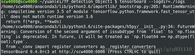
将最后那个网址打开可以看到如下图片所示

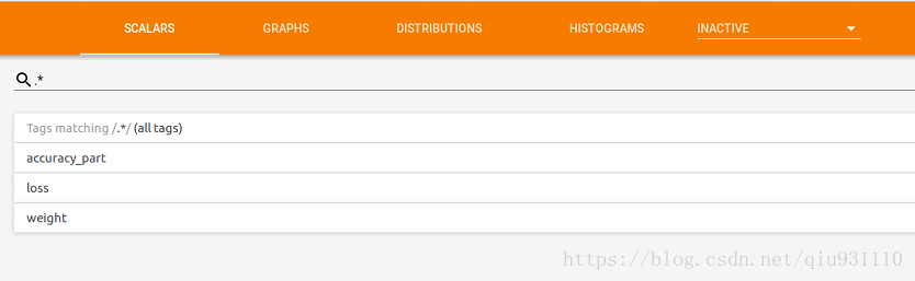
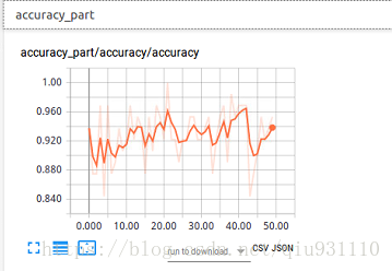
点开accuracy_part

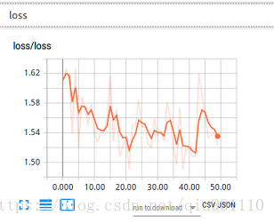
点开loss

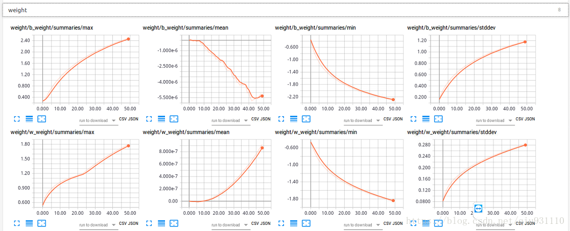
点开weight

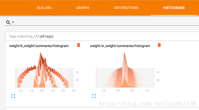
再点开目标栏的histogram

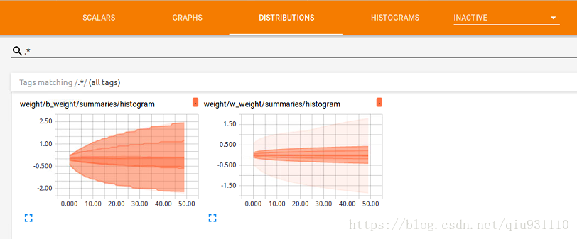
点开distribution