2024年第九届数维杯大学生数学建模挑战赛C 题解题思路1.0版本

题目分析：

问题背景：天然气水合物作为一种高效的清洁后备能源，其资源量评估对未来能源开发极为重要。

具体任务：

0.数据预处理

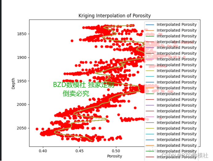
首先将txt中的数据合并到表格里方便后续操作，从Excel文件导入数据，清洗数据，包括删除标记为无效的数据（如-9999）。对其中空缺值使用克里金插值进行补充。

将数据重构成适合分析的格式，为每个钻井分配独立的列（深度、孔隙度、含水合物饱和度）。并进行初始数据的可视化，

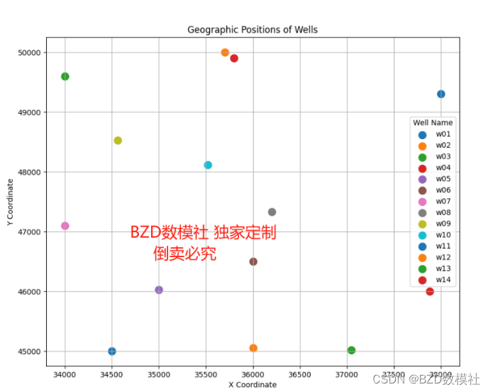
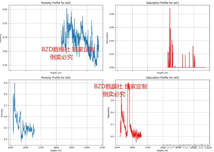
首先我们可以对附件二的地理位置以及部分附件一的数据进行可视化。井位可视化：利用钻井的X、Y坐标在地图上绘制井位，以直观展示钻井的空间分布。钻井数据可视化：选择个别钻井（例如w01和w02），绘制孔隙度和含水合物饱和度随深度的变化曲线图，以了解地质参数的分布特征。 

 

 

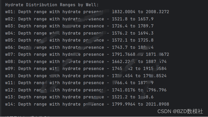
1. 确定天然气水合物资源分布范围。

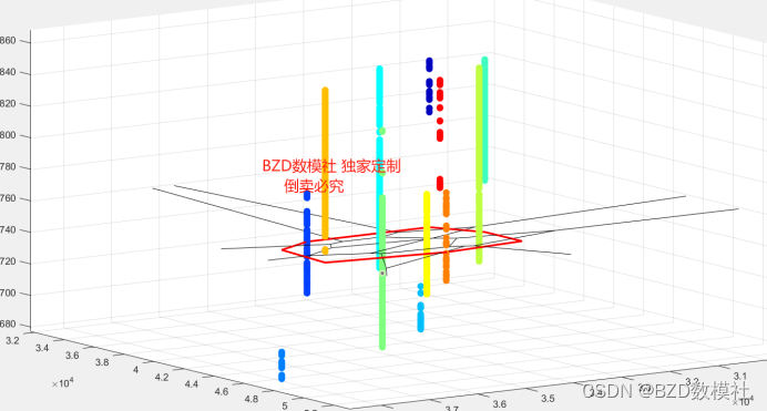
根据钻井数据，确定资源分布的可能边界。这可以通过建立最小外接矩形、Voronoi图或使用空间插值方法（如克里金插值）来完成，以描绘资源的概率分布图。

我们可以绘制单一井的可视化，也可以绘制七个井的可视化，

 

 

最后利用py输出每一个井的高低差即可，并机型可视化表达。 

1. 研究资源参数的概率分布及变化规律。

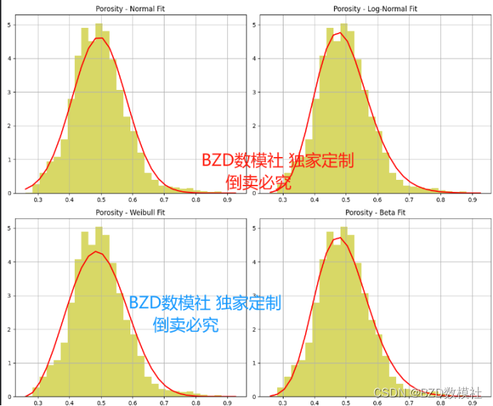
描述性统计分析：计算每个参数的统计描述（均值、中位数、方差等）并绘制其分布（直方图、箱形图）。

概率模型选择：根据数据特性选择合适的概率分布模型（如正态分布、对数正态分布或贝塔分布）来拟合各参数。

地统计学分析：利用克里金方法或其他空间插值技术，研究参数在研究区域内的空间变异性，为参数的空间分布提供模型。

我们实际使用了四种不同的分布拟合情况：正态分布、对数正态分布、Weibull分布和Beta分布，结果均不理想，具体结果如下所示

 

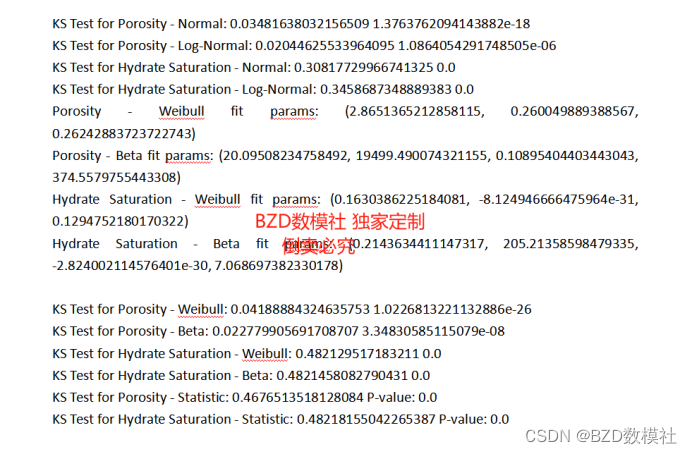
各种分布方式P值都很低，因此，使用混合分布模型，最终得出含有5个高斯分布组件的模型作为最佳模型。 

1. 给出资源量的概率分布估计。

集成模型建立：结合前步骤的地统计模型，计算每个位置的资源量预测值。

蒙特卡洛模拟：利用蒙特卡洛方法对资源量进行随机模拟，以产生资源量的概率分布。

资源量汇总：使用统计方法（如积分或求和）从模拟数据中估计整个区域的总资源量和不确定性。

Q=A*Z*O*S*E 式中，Q为天然气水合物资源量(m3)，A是有效面积m2，Z为有效厚度(m)，O为孔隙度，S为水合物饱和度，E是产气量因子（取值为 155）。 对于每个井位有效面积m2、有效厚度(m)、产气量因子均不一样。 同一井位有效面积m2、有效厚度(m)、产气量因子一样，水合物饱和度、孔隙度，因此对于给出天然气水合物资的概率分布，对于同一井位的只需要看位两者乘积的变化，对于不同井位需要考虑水合物饱和度、孔隙度水合物饱和度、孔隙度四者的乘积，

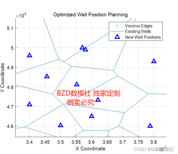
1. 讨论如何安排额外的钻孔位置以优化资源勘探。

数据评估：分析现有钻孔数据，识别数据空白区域或参数高变异性区域。

优化模型：应用地统计学和优化算法（如遗传算法或模拟退火）来选择最佳钻井位置。这些位置应当能最大化潜在资源的发现概率，同时考虑成本效益。

多目标决策分析：考虑多个因素（如成本、资源潜力和环境影响），使用决策支持系统或多标准决策分析来最终确定钻井位置。

1. 使用了Voronoi图中心作为新井位置的候选点，一个有效的策略是通过计算现有Voronoi区域中未充分覆盖的最大区域，并在这些区域中心放置新井。
2. 使用K-均值聚类算法确定新钻井点的位置，可以帮助均匀地分布井位，以便均衡资源勘探的效率
3. 通过蒙特卡洛模拟随机生成新井位置，并计算每种可能位置的效益（如覆盖未探测区域的比例），重复多次以找到最优解。
4. 最大化覆盖模型

这种模型旨在选择井位以最大化地区资源的勘探覆盖率。这可以通过求解一个最大覆盖问题来完成，其中目标是最大化在新井的影响半径内的未探测区域的覆盖。

 

 数据合并 python代码

import pandas as pd
import matplotlib.pyplot as plt
import seaborn as sns

# Load the Excel file
file_path = '附件1：钻井测量数据.xlsx'
data = pd.read_excel(file_path)

# Define the number of wells (from the provided well names)
num_wells = 14

# Create a list for restructured data
well_data_list = []

# Process each well's data block (three columns per well: Depth, Porosity, Saturation)
for i in range(num_wells):
    # Extracting each block, naming columns accordingly
    start_col = 3 * i
    well_data = data.iloc[1:, start_col:start_col+3]
    well_data.columns = ['Depth', 'Porosity', 'Saturation']
    well_data['Well'] = f"w{i+1:02d}"  # Naming wells as w01, w02, ..., w14
    well_data_list.append(well_data)

# Combine all well data into a single DataFrame
combined_well_data = pd.concat(well_data_list, ignore_index=True)

# Convert data types and handle missing values marked as -9999
combined_well_data = combined_well_data.replace(-9999, pd.NA).dropna().astype({'Depth': 'float64', 'Porosity': 'float64', 'Saturation': 'float64'})

# Save the cleaned and combined data to a new Excel file
output_file_path = 'Cleaned_Drilling_Data.xlsx'
combined_well_data.to_excel(output_file_path, index=False)

# Given well positions
well_positions = {
    'w01': (34500, 45000), 'w02': (36000, 45050), 'w03': (37050, 45020),
    'w04': (37880, 46000), 'w05': (35000, 46030), 'w06': (36000, 46500),
    'w07': (34000, 47100), 'w08': (36200, 47330), 'w09': (34560, 48530),
    'w10': (35520, 48120), 'w11': (38000, 49300), 'w12': (35700, 50000),
    'w13': (34000, 49600), 'w14': (35800, 49900)
}

# Create a plot for well positions
plt.figure(figsize=(10, 8))
for well, (x, y) in well_positions.items():
    plt.scatter(x, y, label=well, s=100)

plt.xlabel('X Coordinate')
plt.ylabel('Y Coordinate')
plt.title('Geographic Positions of Wells')
plt.legend(title='Well Name')
plt.grid(True)
plt.show()
# Selecting two wells for detailed visualization: Well w01 and Well w02
selected_wells = ['w01', 'w02']

# Filtering data for the selected wells
selected_data = combined_well_data[combined_well_data['Well'].isin(selected_wells)]

# Plotting data for the selected wells
fig, axes = plt.subplots(nrows=2, ncols=2, figsize=(14, 10), sharex=True)

# Plotting Porosity and Saturation against Depth for each selected well
for i, well in enumerate(selected_wells):
    # Porosity plot
    ax = axes[i, 0]
    well_data = selected_data[selected_data['Well'] == well]
    ax.plot(well_data['Depth'], well_data['Porosity'], label=f"Porosity of {well}")
    ax.set_title(f"Porosity Profile for {well}")
    ax.set_ylabel('Porosity')
    ax.grid(True)

    # Saturation plot
    ax = axes[i, 1]
    ax.plot(well_data['Depth'], well_data['Saturation'], label=f"Saturation of {well}", color='r')
    ax.set_title(f"Saturation Profile for {well}")
    ax.set_ylabel('Saturation')
    ax.grid(True)

# Set common labels
for ax in axes[:, 0]:
    ax.set_xlabel('Depth (m)')
for ax in axes[:, 1]:
    ax.set_xlabel('Depth (m)')

plt.tight_layout()
plt.show()

数据预处理matlab代码

% 假设已经有了钻井的X和Y坐标
well_positions = [
34500, 45000;
36000, 45050;
37050, 45020;
37880, 46000;
35000, 46030;
36000, 46500;
34000, 47100;
36200, 47330;
34560, 48530;
35520, 48120;
38000, 49300;
35700, 50000;
34000, 49600;
35800, 49900
];

% 创建Voronoi图
figure;
voronoi(well_positions(:,1), well_positions(:,2));
title('Voronoi Diagram of Well Locations');
xlabel('X Coordinate');
ylabel('Y Coordinate');
grid on;

% 创建最小外接矩形
k = convhull(well_positions(:,1), well_positions(:,2));
hold on;
plot(well_positions(k,1), well_positions(k,2), 'r-', 'LineWidth', 2);
legend('Voronoi edges', 'Convex hull boundary');
hold off;


well_data = readtable('Cleaned_Drilling_Data.xlsx');

% 添加X和Y坐标到well_data
well_names = {'w01', 'w02', 'w03', 'w04', 'w05', 'w06', 'w07', 'w08', 'w09', 'w10', 'w11', 'w12', 'w13', 'w14'};
for i = 1:length(well_names)
idx = strcmp(well_data.Well, well_names{i});
well_data.X(idx) = well_positions(i, 1);
well_data.Y(idx) = well_positions(i, 2);
end
[XI, YI] = meshgrid(min(well_positions(:,1)):100:max(well_positions(:,1)), ...
min(well_positions(:,2)):100: max(well_positions(:,2)));

% 创建插值网格
[XI, YI] = meshgrid(min(well_data.X):100:max(well_data.X), ...
min(well_data.Y):100:max(well_data.Y));

% 初始化结果矩阵
ZI = zeros(size(XI));

% 对每个网格点进行插值
for i = 1:size(XI, 1)
for j = 1:size(XI, 2)
ZI(i, j) = simpleKriging(well_data.X, well_data.Y, well_data.Saturation, XI(i, j), YI(i, j));
end
end

% 可视化插值结果
figure;
mesh(XI, YI, ZI);
hold on;
plot3(well_data.X, well_data.Y, well_data.Saturation, 'ro');
title('Spatial Interpolation using Simple Kriging');
xlabel('X Coordinate');
ylabel('Y Coordinate');
zlabel('Resource Saturation');
hold off;