三大视觉任务的loss

最新推荐文章于 2025-03-25 13:59:28 发布

CVer儿

最新推荐文章于 2025-03-25 13:59:28 发布

阅读量3.7k

点赞数 1

原文链接：https://mp.weixin.qq.com/s/k7CsGLNoNnSbnAldkafqKQ

版权

pytorch 同时被 2 个专栏收录

61 篇文章

订阅专栏

深度学习

60 篇文章

订阅专栏

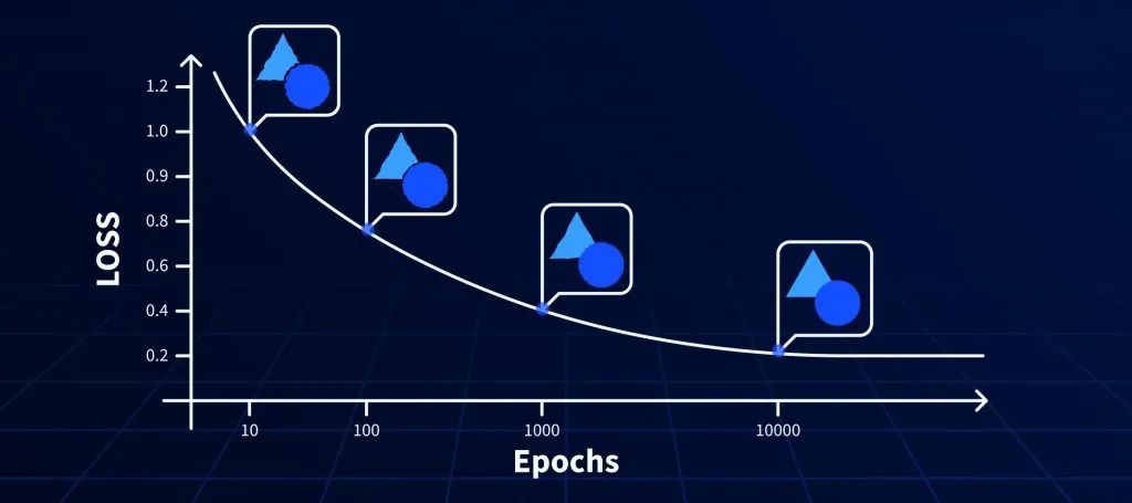
机器学习算法的设计使其可以从错误中“学习”并使用我们提供给他们的训练数据来“更新”自己。但是他们如何量化这些错误呢？这是通过使用“损失函数”来完成的，该函数可以帮助算法了解与基本事实相比，其预测的错误程度。选择合适的损失函数很重要，因为它会影响算法尽快生成最佳结果的能力。

01 基本的损失函数:

1.1 L2 LOSS

这是可用的最基本的损失，也称为MSE Loss。这依赖于两个向量[预测和真实标签]之间的Euclidean距离。
L2 Loss 对异常值非常敏感，因为误差是平方的。

Pytorch 使用范例:

import torchimport numpy as np
a = torch.tensor([[1, 2], [3, 4]], dtype=torch.float)b = torch.tensor([[3, 5], [8, 6]], dtype=torch.float)
loss_fn1 = torch.nn.MSELoss()loss1 = loss_fn1(a.float(), b.float())

1.2 Softmax 函数

分类的损失函数一般都要求算法的每个标量输出输入概率 且和为1。但是预测值并非总是如此，我们可以使用Softmax 函数（非线性函数）将预测值变为概率 且和为1。因此Softmax 函数也称为归一化指数函数，其公式如下：

import torchimport torch.nn.functional as Fx= torch.Tensor( [ [1,2,3,4],[1,2,3,4],[1,2,3,4]])y1= F.softmax(x, dim = 0) #对每一列进行softmaxy2 = F.softmax(x,dim =1) #对每一行进行softmax

图像分类中的损失函数

在图像分类中，经常使用softmax+交叉熵作为损失函数

CROSS-ENTROPY LOSS

Cross Entropy Loss Function交叉熵损失函数是使用对数（loge）的更高级的损失函数。与L2 Loss 相比，这有助于加快对神经网络的训练。
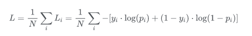
在二分类的情况下交叉熵损失函数被称为BCE Loss，模型最后需要预测的结果只有两种情况，对于每个类别我们的预测得到的概率为和。此时表达式为：

其中：
- —— 表示样本i的label，正类为1，负类为0
- —— 表示样本i预测为正的概率

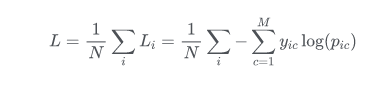
交叉熵（多类别误差）是对二分类的扩展的公式如下。也称为分类交叉熵。

其中：
-    ——类别的数量；
-    ——指示变量（0或1）,如果该类别和样本i的类别相同就是1，否则是0；
-    ——对于观测样本i属于类别  的预测概率。

pytorch 二分类交叉熵 BCE LOSS：

import torchloss = torch.nn.BCEWithLogitsLoss()#preds预测值 如：[0.123,  0.3255, -0.5321]preds= torch.randn(3, requires_grad=True)#target输入是onthot向量，target是真实标签，,可以是[0,0,1,1,0...]多个值为1target = torch.empty(3).random_(2)output = loss(pred, target)

pytorch 多分类交叉熵 CrossEntropy LOSS：

#五分类范例loss = torch.nn.CrossEntropyLoss()preds= torch.randn(3, 5, requires_grad=True)#target输入不是onthot向量，target是真实标签，是稀疏的标签值；tensor([4, 2, 4])target = torch.empty(3, dtype=torch.long).random_(5)output = loss(predsinputs, target)

Label Smoothing

谷歌在交叉熵的基础上，提出了label smoothing（标签平滑）防止模型在训练时过于自信地预测标签，改善泛化能力差的问题。

论文：When Does Label Smoothing Help?

论文链接：https://arxiv.org/pdf/1906.02629.pdf

详细介绍：label smoothing 解读

label smoothing:

label smoothing 是图像分类问题经常会用到的trick，通过对 label 进行 weighted sum，用更新的标签向量来替换传统的ont-hot编码的标签向量能够取得更好的效果: 其中K为多分类的类别总个数，为label smoothing引入的超参数，从上式可以看出，实际上 label smoothing 正如其名称一样，将 label 由原来极端的 one hot 形式转化为较平滑的形式。

class LabelSmoothing(nn.Module):    """NLL loss with label smoothing.    """    def __init__(self, smoothing=0.0):        """Constructor for the LabelSmoothing module.        :param smoothing: label smoothing factor        """        super(LabelSmoothing, self).__init__()        self.confidence = 1.0 - smoothing        self.smoothing = smoothing        # 此处的self.smoothing即我们的epsilon平滑参数。
    def forward(self, x, target):        # 此处x的shape应该是(batch size * class数量)，所以这里在class数量那个维度做了logsoftmax。        logprobs = torch.nn.functional.log_softmax(x, dim=-1)        # 此处的target的shape是(batch size), 应该就是每个training data的数字标签。        nll_loss = -logprobs.gather(dim=-1, index=target.unsqueeze(1))        # 把输出的shape变回(batch size)        nll_loss = nll_loss.squeeze(1)        # 在第二个维度取均值的话，应该就是对每个x，所有类的logprobs取了平均值。        smooth_loss = -logprobs.mean(dim=-1)        loss = self.confidence * nll_loss + self.smoothing * smooth_loss        return loss.mean()

目标检测中的损失函数

目标检测的损失函数一般由classification loss和bounding box regression loss组成，这部分我们以YOLOv5为例介绍目标检测中的损失函数因为它包括了多数情况。详细介绍可以看我们之前的教程：YOLOv5从入门到部署之：网络和损失函数

分类损失

首先是分类损失：YOLOv5 采用了BECLogits 损失函数计算objectness score的损失，class probability score采用了交叉熵损失函数(BCEclsloss)，这两种loss 和上述介绍的图像分类交叉熵损失基本一致，区别在于目标检测中需要有一个二分类区分是否为背景的loss，以及判断目标的类别多分类损失。

objectness loss:

class loss：

Focal Loss

在分类损失中YOLOV5还提供 Focal Loss 来缓解样本的不平衡，何凯明团队在他们的论文Focal Loss for Dense Object Detection 提出来的损失函数，主要是为了解决one-stage目标检测中正负样本比例严重失衡的问题。该损失函数降低了大量简单负样本在训练中所占的权重，也可理解为一种困难样本挖掘。

Focal Loss是在交叉熵损失上进行改进，普通的交叉熵对于正样本而言，输出概率越大损失越小。对于负样本而言，输出概率越小则损失越小。此时的损失函数在大量简单样本的迭代过程中比较缓慢且可能无法优化至最优。那么Focal loss是怎么改进的呢？首先在原有的基础上加了一个因子，其中gamma>0使得减少易分类样本的损失。使得更关注于困难的、错分的样本。此外，加入平衡因子alpha，用来平衡正负样本本身的比例不均：文中alpha取0.25，即正样本要比负样本占比小，这是因为负例易分。

class FocalLoss(nn.Module):    # Wraps focal loss around existing loss_fcn(), i.e. criteria = FocalLoss(nn.BCEWithLogitsLoss(), gamma=1.5)    def __init__(self, loss_fcn, gamma=1.5, alpha=0.25):        super(FocalLoss, self).__init__()        self.loss_fcn = loss_fcn  # must be nn.BCEWithLogitsLoss()        self.gamma = gamma        self.alpha = alpha        self.reduction = loss_fcn.reduction        self.loss_fcn.reduction = 'none'  # required to apply FL to each element
    def forward(self, pred, true):        loss = self.loss_fcn(pred, true)        # p_t = torch.exp(-loss)        # loss *= self.alpha * (1.000001 - p_t) ** self.gamma  # non-zero power for gradient stability
        # TF implementation https://github.com/tensorflow/addons/blob/v0.7.1/tensorflow_addons/losses/focal_loss.py        pred_prob = torch.sigmoid(pred)  # prob from logits        p_t = true * pred_prob + (1 - true) * (1 - pred_prob)        alpha_factor = true * self.alpha + (1 - true) * (1 - self.alpha)        modulating_factor = (1.0 - p_t) ** self.gamma        loss *= alpha_factor * modulating_factor
        if self.reduction == 'mean':            return loss.mean()        elif self.reduction == 'sum':            return loss.sum()        else:  # 'none'            return loss

回归损失

接下来是最重要的回归损失，YOLOv1采用的回归框loss更像是MSE，YOLOv1是，而对w和h分别取平方根做差，再求平方，用以消除一些物体大小不均带来的不利。YOLOv2和YOLOv3则利用 , 将框大小的影响放在前面作为系数，连x和y部分也一块考虑了进去。

YOLOv4作者认为YOLOv1-v3建立的类MSE损失是不合理的。因为MSE的四者是需要解耦独⽴的，但实际上这四者并不独⽴，应该需要⼀个损失函数能捕捉到它们之间的相互关系。因此引入了IOU系列。经过其验证，GIOU，DIOU, CIOU，最终作者发现CIOU效果最好，另外YOLOv5采用 GIOU。

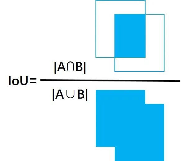
IOU

IoU就是我们所说的交并比，就是两个图形面积的交集和并集的比值

GIOU Loss

IOU的缺陷在于预测的检测框如果和真实物体的检测框没有重叠（没有交集）的话，我们从IoU的公式可以看出，IoU始终为0且无法优化，也就是如果算法一开始检测出来的框很离谱，根本没有和真实物体发生交集的话，算法无法优化。因此GIOU被提出：

论文：Generalized Intersection over Union: A Metric and A Loss for Bounding Box Regression

论文链接：https://arxiv.org/pdf/1902.09630.pdf

GIOU:

上面公式的意思将两个任意框A，B，我们找到一个最小的封闭形状C，让C可以把A，B包含在内，接着计算C中没有覆盖A和B的面积占C总面积的比值，然后用A与B的IoU减去这个比值。与IoU类似，GIoU也可以作为一个距离，loss可以用

GIoU代码：YOLOv5 的 general.py bbox_iou 函数返回值是GIoU值iou = inter / union # iou inter是A和B的相交面积，union是A和B的面积之和，计算A和B的IOU

if GIoU or DIoU or CIoU:  # 可以选择三种IOU ，yolov5默认采用GIOU    cw = torch.max(b1_x2, b2_x2) - torch.min(b1_x1, b2_x1)  # convex (smallest enclosing box) width      ch = torch.max(b1_y2, b2_y2) - torch.min(b1_y1, b2_y1)  # convex height      if GIoU:  # Generalized IoU https://arxiv.org/pdf/1902.09630.pdf          c_area = cw * ch + 1e-16  # convex area  计算公式里的C 就是能够包含A和B的最小矩形面积          return iou - (c_area - union) / c_area  # GIoU

GIoU Loss代码 : 在compute_loss 函数

# Regression  pxy = ps[:, :2].sigmoid() * 2. - 0.5      #预测框的中心点  pwh = (ps[:, 2:4].sigmoid() * 2) ** 2 * anchors[i]   #预测框的hw  pbox = torch.cat((pxy, pwh), 1).to(device)  # predicted box  iou = bbox_iou(pbox.T, tbox[i], x1y1x2y2=False, CIoU=True)  # iou(prediction, target)  lbox += (1.0 - iou).mean()  # iou loss       giou_loss = 1- giou

Classloss和Obj loss 代码：在compute_loss 函数 obj loss 采用BEC Logits loss，class loss 采用BCEcls loss二分类交叉熵损失。

    # Objectness      tobj[b, a, gj, gi] = (1.0 - model.gr) + model.gr * iou.detach().clamp(0).type(tobj.dtype)  # iou ratio  
    # Classification      if model.nc > 1:  # cls loss (only if multiple classes)          t = torch.full_like(ps[:, 5:], cn, device=device)  # targets          t[range(n), tcls[i]] = cp          lcls += BCEcls(ps[:, 5:], t)  # BCE  
    # Append targets to text file      # with open('targets.txt', 'a') as file:      #     [file.write('%11.5g ' * 4 % tuple(x) + '\n') for x in torch.cat((txy[i], twh[i]), 1)]  
lobj += BCEobj(pi[..., 4], tobj) * balance[i]  # obj loss

图像分割中的损失函数

图像分割可以定义为像素级别的分类任务。图像由各种像素组成，这些像素组合在一起定义了图像中的不同元素，因此将这些像素分类为一类元素的方法称为语义图像分割。

大家可以看这篇关于图像分割的损失函数综述

论文：A survey of loss functions for semantic segmentation

论文地址：https://arxiv.org/pdf/2006.14822.pdf

代码地址：https://github.com/shruti-jadon/Semantic-Segmentation-Loss-Functions

在文中，总结了15种基于图像分割的损失函数。被证明可以在不同领域提供最新技术成果。这些损失函数可大致分为4类：基于分布的损失函数，基于区域的损失函数，基于边界的损失函数和基于复合的损失函数，如下表所示：

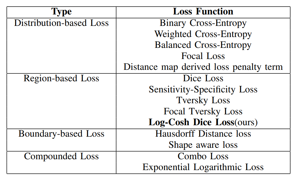
基于分布的损失函数：

基于分布的损失函数，主要有Binary Cross-Entropy, Weighted Cross-Entropy, Balanced Cross-Entropy Focal Loss, Distance map derived loss, penalty term。其中Binary Cross-Entropy二进制交叉熵损失和Focal Loss我们在上文中介绍了，我们主要介绍Weighted Cross-Entropy加权交叉熵以及损失平衡交叉熵损失函数。

Weighted Cross-Entropy 加权交叉熵损失函数

加权交叉熵损失函数只是在交叉熵Loss的基础上为每一个类别添加了一个权重参数为正样本加权。设置减少假阴性，设置减少假阳性。这样相比于原始的交叉熵Loss，在样本数量不均衡的情况下可以获得更好的效果。

公式如下所示：

pytroch 代码：

   class WeightedCrossEntropyLoss(torch.nn.CrossEntropyLoss):   """   Network has to have NO NONLINEARITY!   """   def __init__(self, weight=None):       super(WeightedCrossEntropyLoss, self).__init__()       self.weight = weight
   def forward(self, inp, target):       target = target.long()       num_classes = inp.size()[1]
       i0 = 1       i1 = 2
       while i1 < len(inp.shape): # this is ugly but torch only allows to transpose two axes at once           inp = inp.transpose(i0, i1)           i0 += 1           i1 += 1
       inp = inp.contiguous()       inp = inp.view(-1, num_classes)
       target = target.view(-1,)       wce_loss = torch.nn.CrossEntropyLoss(weight=self.weight)
       return wce_loss(inp, target)

Balanced Cross-Entropy 平衡交叉熵损失函数

平衡交叉熵损失函数与加权交叉熵损失函数类似，但平衡交叉熵损失函数对负样本也进行加权。公式如下:

基于区域的损失函数：

基于区域的loss旨在最大程度地减少失配或最大化ground truth G与预测的分割S之间的重叠区域。主要的损失函数是Dice Loss。

Dice系数是计算机视觉界广泛使用的度量标准，用于计算两个图像之间的相似度。在2016年的时候，它也被改编为损失函数，称为Dice Loss，公式如下：此处，在分子和分母中添加1以确保函数在诸如y = 0的极端情况下的确定性。Dice Loss使用与样本极度不均衡的情况，如果一般情况下使用Dice Loss会回反向传播有不利的影响，使得训练不稳定。

class SoftDiceLoss(nn.Module):   def __init__(self, apply_nonlin=None, batch_dice=False, do_bg=True, smooth=1.,                square=False):       """       paper: https://arxiv.org/pdf/1606.04797.pdf       """       super(SoftDiceLoss, self).__init__()
       self.square = square       self.do_bg = do_bg       self.batch_dice = batch_dice       self.apply_nonlin = apply_nonlin       self.smooth = smooth
   def forward(self, x, y, loss_mask=None):       shp_x = x.shape
       if self.batch_dice:           axes = [0] + list(range(2, len(shp_x)))       else:           axes = list(range(2, len(shp_x)))
       if self.apply_nonlin is not None:           x = self.apply_nonlin(x)
       tp, fp, fn = get_tp_fp_fn(x, y, axes, loss_mask, self.square)
       dc = (2 * tp + self.smooth) / (2 * tp + fp + fn + self.smooth)
       if not self.do_bg:           if self.batch_dice:               dc = dc[1:]           else:               dc = dc[:, 1:]       dc = dc.mean()
       return -dc

基于边界的损失函数

基于边界的损失是一种新型的损失函数，旨在最小化地面真实情况和预测的分段之间的距离。

Shape-aware Loss

顾名思义，Shape-aware Loss考虑了形状。通常，所有损失函数都在像素级起作用，Shape-aware Loss会计算平均点到曲线的欧几里得距离，即预测分割到ground truth的曲线周围点之间的欧式距离，并将其用作交叉熵损失函数的系数，具体定义如下：（CE指交叉熵损失函数）

class DistBinaryDiceLoss(nn.Module):   """   Distance map penalized Dice loss   Motivated by: https://openreview.net/forum?id=B1eIcvS45V   Distance Map Loss Penalty Term for Semantic Segmentation           """   def __init__(self, smooth=1e-5):       super(DistBinaryDiceLoss, self).__init__()       self.smooth = smooth
   def forward(self, net_output, gt):       """       net_output: (batch_size, 2, x,y,z)       target: ground truth, shape: (batch_size, 1, x,y,z)       """       net_output = softmax_helper(net_output)       # one hot code for gt       with torch.no_grad():           if len(net_output.shape) != len(gt.shape):               gt = gt.view((gt.shape[0], 1, *gt.shape[1:]))
           if all([i == j for i, j in zip(net_output.shape, gt.shape)]):               # if this is the case then gt is probably already a one hot encoding               y_onehot = gt           else:               gt = gt.long()               y_onehot = torch.zeros(net_output.shape)               if net_output.device.type == "cuda":                   y_onehot = y_onehot.cuda(net_output.device.index)               y_onehot.scatter_(1, gt, 1)              gt_temp = gt[:,0, ...].type(torch.float32)       with torch.no_grad():           dist = compute_edts_forPenalizedLoss(gt_temp.cpu().numpy()>0.5) + 1.0       # print('dist.shape: ', dist.shape)       dist = torch.from_numpy(dist)
       if dist.device != net_output.device:           dist = dist.to(net_output.device).type(torch.float32)              tp = net_output * y_onehot       tp = torch.sum(tp[:,1,...] * dist, (1,2,3))              dc = (2 * tp + self.smooth) / (torch.sum(net_output[:,1,...], (1,2,3)) + torch.sum(y_onehot[:,1,...], (1,2,3)) + self.smooth)
       dc = dc.mean()
       return -dc