圆周运动、一般曲线运动、阿基米德螺旋线

恒长旋转向量的导数

一个恒长旋转向量求导后得到的向量的方向与原向量相比，逆时针旋转了 $90^{\circ }$ ，而求导后得到的向量的长度与旋转角速度有关。

证明

例如 $\vec{a}=(cos\theta ,sin\theta )$
1、对 $\theta$ 求导
$$\frac{d\vec{a}}{d\theta }=(-sin\theta ,cos\theta )=[cos(\theta +\frac{\pi }{2}),sin(\theta +\frac{\pi }{2})]$$
结论：
$\frac{d\vec{a}}{d\theta }$ 与 $\vec{a}$ 相比，在方向上逆时针旋转了 90°，长度不变

---

2、对 t 求导
$\theta$ 是关于 $t$ 的函数，$\theta =w\cdot t或\theta =w(t)\cdot t$前者角速度恒定，后者角速度是关于时间的函数。
$$\frac{d\vec{a}}{dt}=\frac{d\vec{a}}{d\theta }\cdot \frac{d\theta }{dt}=[\frac{d\theta }{dt}\cdot cos(\theta +\frac{\pi }{2}),\frac{d\theta }{dt}\cdot sin(\theta +\frac{\pi }{2})]$$
结论：
所以， $\frac{d\vec{a}}{dt}$ 与 $\vec{a}$ 相比，在方向上逆时针旋转了 90° ，在长度上变为原来的 $w$ 倍，如果 $\vec{a}$ 作变速圆周运动，$\frac{d\vec{a}}{dt}$ 的长度将会随时间变化。

圆周运动中角速度和线速度的关系

一个质点以原点为圆心作圆周运动，设它的位移由 $\overrightarrow{r_1}$ 变成 $\overrightarrow{r_2}$ ，如下图所示

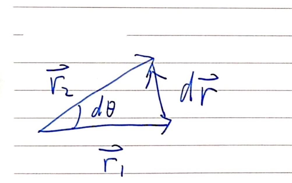
$d\vec{r}$ 是位移的变化量，$d\theta$ 是弧度增量。
$$\begin{gathered} d\vec{r}=\overrightarrow{r_2}-\overrightarrow{r_1} \\ |\overrightarrow{r_1}|=|\overrightarrow{r_2}|=r \end{gathered}$$
当 $d\theta$ 很小时， $|d\vec{r}|\approx 弧长$ 根据 $弧度=\frac{弧长}{半径}$ ，可得 $d\theta =\frac{|d\vec{r}|}{r}$，使用标量表示：$dr=d\theta \cdot r$ ，方程两边同时除以 dt ，得: $\frac{dr}{dt}=r\cdot \frac{d\theta }{dt}$，则得到：$v=w\cdot r$

这只是大小关系，考虑方向，使用叉乘，$\vec{v}=\vec{w}\times \vec{r}$

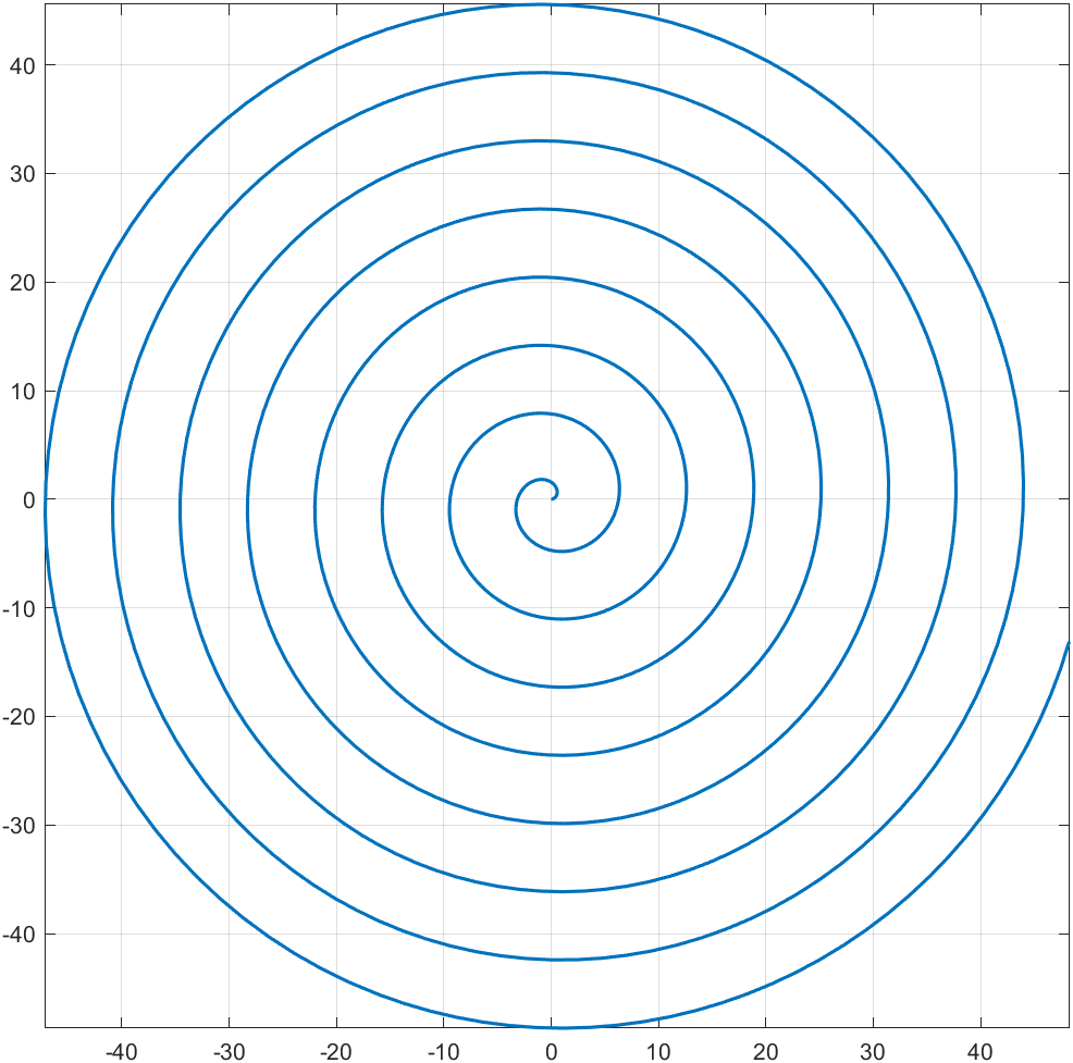
阿基米德螺旋线

阿基米德螺旋线方程

阿基米德螺旋线的极坐标方程为：$r=a\theta (a>0)$ 这表示极径与 $\theta$ 是线性关系，成正比。
它的参数方程为：
$$\{\begin{array}{l}x=r\cdot cos\theta =a\theta \cdot cos\theta \\ y=r\cdot sin\theta =a\theta \cdot sin\theta \end{array}$$
试图消去参数
$$x^2+y^2=(a\theta {)}^2\cdot (si{n}^2\theta +co{s}^2\theta )=(a\theta {)}^2其中，\theta =arctan(\frac{y}{x})$$
这个方程无法化为显函数的形式，所以，最好用极坐标方程或参数方程来表示。我们以 $\theta$ 为参数，用 matlab 画出它的图像。

syms theta
a=1;
r=a*theta;
x=r*cos(theta);
y=r*sin(theta);
fplot(x,y,[0,50],'LineWidth',1.5);
grid on
axis square

螺旋线的时间导数

设 $\vec{r}$ 为螺旋线的位移，$\frac{d\vec{r}}{dt}=\frac{d\vec{r}}{d\theta }\cdot \frac{d\theta }{dt}$ .

可见，$\vec{r}$ 对时间求导只是对 $\theta$ 求导后乘上一个系数 $\frac{d\theta }{dt}$ 而已，所以我们研究对 $\theta$ 的导数，而不是对 $t$ 的导数。

对螺旋线的参数方程求导

syms a theta
x=a*theta*cos(theta);
y=a*theta*sin(theta);
dx=diff(x,theta)
dy=diff(y,theta)

结果如下

 
dx =
 
a*cos(theta) - a*theta*sin(theta)
 
 
dy =
 
a*sin(theta) + a*theta*cos(theta)
 
>> 

这可以看成是两个向量的合成，分别为
$$(a\cdot cos\theta ,a\cdot sin\theta )$$
和
$$(-a\theta \cdot sin\theta ,a\theta \cdot cos\theta )=[a\theta \cdot cos(\theta +\frac{\pi }{2}),a\theta \cdot sin(\theta +\frac{\pi }{2})]$$
分别令
$$\{\begin{array}{l}\overrightarrow{e_t}=[a\theta \cdot cos(\theta +\frac{\pi }{2}),a\theta \cdot sin(\theta +\frac{\pi }{2})]\\ \overrightarrow{e_n}=(a\cdot cos\theta ,a\cdot sin\theta )\end{array}$$

$$\{\begin{array}{l}\overrightarrow{v_t}=\frac{d\theta }{dt}\cdot \overrightarrow{e_t}=w\cdot \overrightarrow{e_t}\\ \overrightarrow{v_n}=\frac{d\theta }{dt}\cdot \overrightarrow{e_n}=w\cdot \overrightarrow{e_n}\end{array}$$
其中，$\overrightarrow{v_n}$ 的方向沿着半径向外，是法向速度， $\overrightarrow{v_t}$ 沿着切线，与$\overrightarrow{v_n}$ 垂直，总是指向逆时针方向，是切向速度。

可以看出 $w$ 恒定时，切向速度随着 $\theta$ 的增大而增大，法向速度恒定，此时质点一方面绕着原点作圆周运动，线速度越来越大；另一方面，又以恒定的速度远离原点。

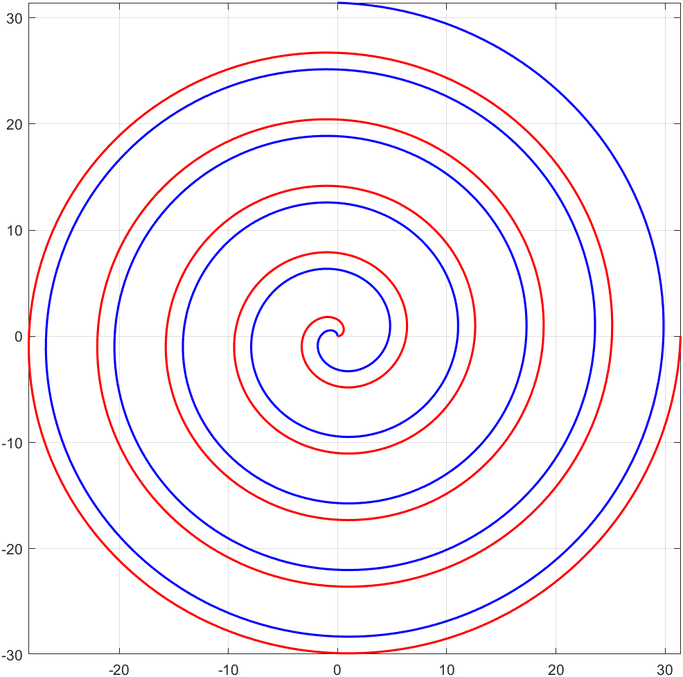
切向速度的规律

这个切向速度与原来的螺旋线方程比起来有什么规律呢？
螺旋线参数方程
$$\{\begin{array}{l}x=r\cdot cos\theta =a\theta \cdot cos\theta \\ y=r\cdot sin\theta =a\theta \cdot sin\theta \end{array}$$
切向速度
$$\overrightarrow{v_t}=[a\theta \cdot cos(\theta +\frac{\pi }{2}),a\theta \cdot sin(\theta +\frac{\pi }{2})]$$
可以发现，切向速度与螺旋线方程比起来就是逆时针旋转了 $\frac{\pi }{2}$ 而已。

使用 matlab 画出切向速度的图像

clc;
clear;
close all;

syms theta
a=1;
x=a*theta*cos(theta+pi/2);
y=a*theta*sin(theta+pi/2);
fplot(x,y,[0,pi*2*5],'LineWidth',1.5,'Color','b');%画出切向速度，蓝色
grid on
axis square
hold on
x=a*theta*cos(theta);
y=a*theta*sin(theta);
fplot(x,y,[0,pi*2*5],'LineWidth',1.5,'Color','r');%画出阿基米德螺旋线，红色

切向速度可以使用 $\vec{v}=\vec{w}\times \vec{r}$ 的公式。（合速度不行）

1、使用方程组得到 $v_t$（$v_t$ 的标量，即它的大小）
$$\{\begin{array}{l}\overrightarrow{e_t}=[a\theta \cdot cos(\theta +\frac{\pi }{2}),a\theta \cdot sin(\theta +\frac{\pi }{2})]\\ \overrightarrow{e_n}=(a\cdot cos\theta ,a\cdot sin\theta )\end{array}$$

$$\{\begin{array}{l}\overrightarrow{v_t}=\frac{d\theta }{dt}\cdot \overrightarrow{e_t}=w\cdot \overrightarrow{e_t}\\ \overrightarrow{v_n}=\frac{d\theta }{dt}\cdot \overrightarrow{e_n}=w\cdot \overrightarrow{e_n}\end{array}$$
则标量方程为：
$$\{\begin{array}{l}{v}_t=wa\theta =w^{2}at\\ v_n=wa\end{array}$$
2、使用 $\vec{v}=\vec{w}\times \vec{r}$ 得到 $v_t$
$$v_t=wr=w\cdot a\theta =wa\cdot wt=w^{2}at$$
这两种方式得到的 $v_t$ 一样，可见，对于任意的曲线运动，它的切向速度总是适用 $\vec{v}=\vec{w}\times \vec{r}$ ，但是它的合速度不能盲目地使用这个公式。

题外话——蚊香线

两条互差 180° 得阿基米德螺旋线就是蚊香得形状

clc;
clear;
close all;

syms theta
a=1;
x=a*theta*cos(theta+pi);
y=a*theta*sin(theta+pi);
fplot(x,y,[0,pi*2*5],'LineWidth',1.5,'Color','b');
grid on
axis square
hold on
x=a*theta*cos(theta);
y=a*theta*sin(theta);
fplot(x,y,[0,pi*2*5],'LineWidth',1.5,'Color','r');

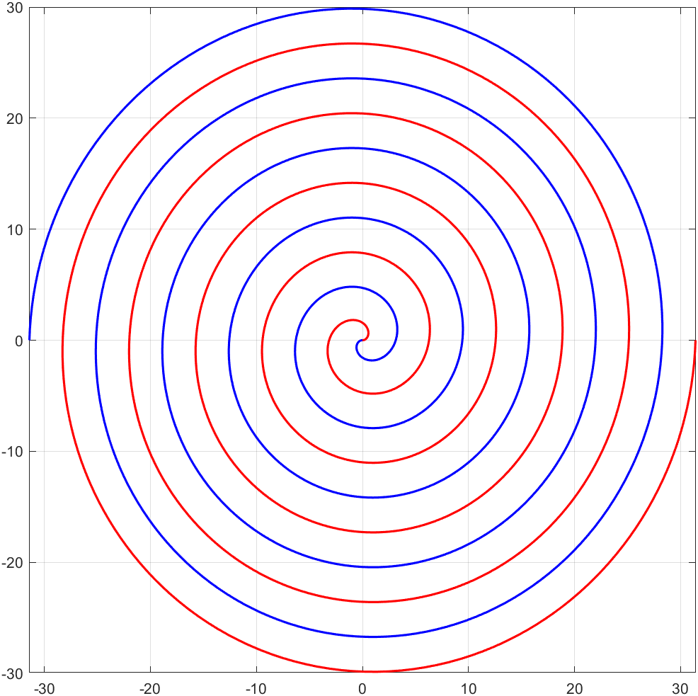
在一个平面上切割两条阿基米德螺旋线，然后横着切两刀，剩下的部分丢掉，把要的部分扒开就是两盘蚊香了。