LQR制导

LQR制导

引言

在ardupilot中固定翼飞机横航向位置控制（制导律）采用L1制导律，最近想将一些其他的控制理论用于ardupilot代码中，通过ardupilot论坛，看到已经有大佬曾经将L1用于固定翼制导律，并且已经向ardupilot官方github中pr了，但是由于pr的方式有误，被官方驳回了，但是我还是通过连接查到了大佬的代码，并且自己尝试了一下，已经编译通过并进行了仿真，后面我会把链接放到文章结尾。欢迎大家一起来讨论。

LQR理论

LQR（线性二次调节器）是一种最优控制方法，网上已经有很多关于其理论的介绍，在这里就不多介绍。核心思想就是通过给定合理的状态权重矩阵Q和控制权重矩阵R，求解最优控制量u，这里的控制变量为横向将速度$a_{scmd}$,状态量为位置误差$d$及其导数及其导数$v_d$,即$[d,v_d{]}^T$,LQR理论部分可以参考博客lqr理论。
根据LQR理论以及参考的论文，可总结为以下几点：
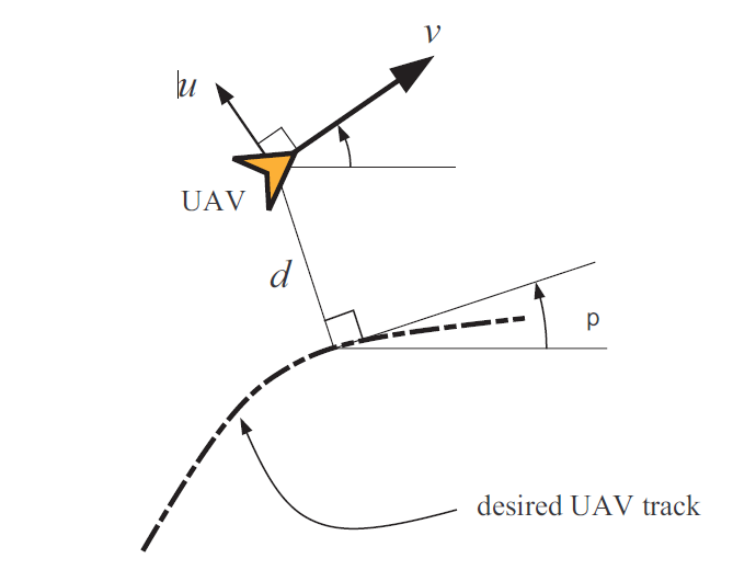
固定翼飞机在空中飞行的运动方程为：

$$\dot{d}=vsin(\psi -{\psi }_p)\text{\hspace{1em}(theory-1)}$$
其中，d为飞机速度方向与期望路径方向的直线距离，$\psi$为航向角，${\psi }_p$为期望航向角。
侧向加速度$a_{scmd}$为：
$$a_{scmd}=u={\dot{v}}_d=v\dot{\psi }\text{\hspace{1em}(theory-2)}$$
状态方程为：
$$\dot{x}=Ax+Bu\text{\hspace{1em}(theory-3)}$$
其中：
$$x=\left[\begin{array}{c}d\\ v_d\end{array}\right],根据公式(2)可得:A=\left[\begin{array}{cc}0& 1\\ 0& 0\end{array}\right],B=\left[\begin{array}{c}0\\ 1\end{array}\right]$$
有了AB阵便可按照LQR的步骤进行求解：
（1）选取参考矩阵Q,R。
（2）根据Riccati方程得到矩阵P。
（3）求u。
首先定义Q矩阵和R矩阵：
我们假设：
$$R=1\text{\hspace{1em}(theory-4)}$$
$$Q=\left[\begin{array}{cc}{q}_1^2& 0\\ 0& q_2^2\end{array}\right]\text{\hspace{1em}(theory-5)}$$
然后定义矩阵P：
$$P=\left[\begin{array}{cc}{p}_{11}& p_{12}\\ p_{21}& p_{22}\end{array}\right]\text{\hspace{1em}(theory-6)}$$
根据Riccati方程可知A,B,Q,R的关系：
$$A^{T}P+PA-PB{R}^{-1}{B}^T+Q=0\text{\hspace{1em}(theory-7)}$$
根据式7可得P和Q元素的对应关系：
$$p_{12}=q_1\text{\hspace{1em}(theory-8)}$$
$$p_{22}=\sqrt{2q_1+q_2^2}\text{\hspace{1em}(theory-9)}$$
$$p_{11}=q_1\sqrt{2q_1+q_2^2}\text{\hspace{1em}(theory-10)}$$
最优控制给出：
$$u=-R^{-1}{B}^{T}Px\text{\hspace{1em}(theory-11)}$$
上文已经退出P和Q的关系，所以可以将控制量$u$以已知量R,B,P表示，最终得出：
$$a_{scmd}=u=-[q_{1}d+\sqrt{2q_1+q_2^2}\cdot v_d]\text{\hspace{1em}(theory-12)}$$
$$q_1^2=\frac{d_b}{d_b-d},q_2^2=1\text{\hspace{1em}(theory-13)}$$
所以得：
$$a_{scmd}=-[\sqrt{|\frac{d_b}{d_b-d}|}d+\sqrt{2\sqrt{|\frac{d_b}{d_b-d}}|+1}\cdot v_d\text{\hspace{1em}(theory-14)}$$

部分代码展示

代码与理论的对应关系：
$$v_d=Vcos(\psi -\psi )\text{\hspace{1em}(code-1)}$$
$$p_{12}=\frac{q_1}{cos(\psi -{\psi }_p)}\text{\hspace{1em}(code-2)}$$
$$p_{22}=\frac{\sqrt{2p_{12}+q_2^2}}{cos(\psi -{\psi }_p)}\text{\hspace{1em}(code-3)}$$
$$a_{csd}=-(d\cdot p_{12}\cdot cos(\psi -\psi )+p_{22}\cdot v_d\cdot cos(\psi -\psi ))\text{\hspace{1em}(code-4)}$$
将（2）与（4）带入（4）可得：
$$a_{scmd}=-[q_{1}d+\sqrt{2p_{12}+q_2^2}\cdot v_d]\text{\hspace{1em}(code-5)}$$
接下来说下q的选取：
在代码中，自适应增益$q_1$为：
$$q_1=\sqrt{K\cdot |d|}\text{\hspace{1em}(code-6)}$$
$q_2$是自定义的值，在论文中定义$q_2^2=1$，在代码中$q_2$为地面站可调节的参数，默认值同论文。
代码：

//更新LQR控制用于航点导航
void AP_LQR_Control::update_waypoint(const struct Location &prev_WP, const struct Location &next_WP, float dist_min)
{
    //定义当前位置
    struct Location _current_loc;

    uint32_t now = AP_HAL::micros();
    float dt = (now - _last_update_waypoint_us) * 1.0e-6f;
    if(dt > 0.1f){
        dt = 0.1f;
    }
    _last_update_waypoint_us = now;

    //获取当前你位置和速度
    if(_ahrs.get_position(_current_loc) == false){
        //如果没有GPS信号，维持上一次航向角
        _data_is_stale = true;
        return;
    }

    Vector2f _groundspeed_vector = _ahrs.groundspeed_vector();

    //更新_target_bearing_cd(航向角)
    _target_bearing_cd = _current_loc.get_bearing_to(next_WP);

    //计算地速
    float groundSpeed = _groundspeed_vector.length();
    if(groundSpeed < 0.1f){
        groundSpeed = 0.1f;
        _groundspeed_vector = Vector2f(cosf(get_yaw_rad()), sinf(get_yaw_rad())) * groundSpeed;
    }

    //计算NE坐标系下B相对于A点的距离
    Vector2f AB = prev_WP.get_distance_NE(next_WP);

    //检查AB的长度，判断追踪距离是否太短
    if(AB.length() < 1.0e-6f){
        AB = _current_loc.get_distance_NE(next_WP);
        if(AB.length() < 1.0e-6f){
            AB = Vector2f(cosf(get_yaw_rad()), sinf(get_yaw_rad()));
        }
    }

    //单位化
    AB.normalize();

    //计算飞机相对于A点NE位置
    Vector2f A_air = prev_WP.get_distance_NE(_current_loc);

    //计算目标追踪
    _crosstrack_error = (A_air % AB)/(AB.length());
    _crosstrack_error = -_crosstrack_error;

    //计算自适应增益
    //exp为以e为底的指数函数
    float q1 = sqrtf(float(exp(_k_val * abs(_crosstrack_error))));

    //计算路径上的跟踪速度
    float si = get_gs_angle_cd() * 0.01f;
    float si_p = (prev_WP.get_bearing_to(next_WP)) * 0.01;
    float temp_sin = sinf(radians(si - si_p));
    float v_d = groundSpeed * temp_sin;

    float cos_term = cosf(radians(si - si_p));

    if(fabs(cos_term) < 0.01)
    {
        if(cos_term < 0 ){
            cos_term = float(-0.01);
        }else{
            cos_term = float(0.01);
        }
    }

    float p12 = float(q1/fabs(cos_term));
    float p22 = sqrtf((float)(2*p12 + _q2_val)) / (cos_term);

    //基于当前状态和自适应增益计算横向加速度
    float u = -(_crosstrack_error * p12 * cosf(radians(si - si_p)) + p22 * v_d * cosf(radians(si - si_p)));

    _latAccDem = u;
    _bearing_error = radians(si - si_p);
    _nav_bearing = radians(si_p);

    //在航路点跟踪期间，航路点捕获状态始终为false
    _WPcircle = false;
    _data_is_stale = false;//使用当前航路点数据正确更新状态

}

reference

1. https://github.com/ArduPilot/ardupilot/pull/10037/files
2. Ratnoo A, Sujit P B, Kothari M. Adaptive optimal path following for high wind flights[J]. IFAC Proceedings Volumes, 2011, 44(1): 12985-12990.