


这个单子主要难点在神经网络的搭建,因为自己神经网络没有学过多少,差不多花了两天去寻找以及搭建神经网络,多多少少有点入门,还有就是通过箱型图判断缺失值,其余的都是旧知识,一些分类算法的应用。
import pandas as pd
import matplotlib.pyplot as plt
%matplotlib inline
import warnings
warnings.filterwarnings('ignore')
test=pd.read_csv('CMP3751M_CMP9772M_ML_Assignment 2-dataset-nuclear_plants_final.csv')
test.head()
| Status | Power_range_sensor_1 | Power_range_sensor_2 | Power_range_sensor_3 | Power_range_sensor_4 | Pressure _sensor_1 | Pressure _sensor_2 | Pressure _sensor_3 | Pressure _sensor_4 | Vibration_sensor_1 | Vibration_sensor_2 | Vibration_sensor_3 | Vibration_sensor_4 | |
|---|---|---|---|---|---|---|---|---|---|---|---|---|---|
| 0 | Normal | 4.5044 | 0.7443 | 6.3400 | 1.9052 | 29.5315 | 0.8647 | 2.2044 | 6.0480 | 14.4659 | 21.6480 | 15.3429 | 1.2186 |
| 1 | Normal | 4.4284 | 0.9073 | 5.6433 | 1.6232 | 27.5032 | 1.4704 | 1.9929 | 5.9856 | 20.8356 | 0.0646 | 14.8813 | 7.3483 |
| 2 | Normal | 4.5291 | 1.0199 | 6.1130 | 1.0565 | 26.4271 | 1.9247 | 1.9420 | 6.7162 | 5.3358 | 11.0779 | 25.0914 | 9.2408 |
| 3 | Normal | 5.1727 | 1.0007 | 7.8589 | 0.2765 | 25.1576 | 2.6090 | 2.9234 | 6.7485 | 1.9017 | 1.8463 | 28.6640 | 4.0157 |
| 4 | Normal | 5.2258 | 0.6125 | 7.9504 | 0.1547 | 24.0765 | 3.2113 | 4.4563 | 5.8411 | 0.5077 | 9.3700 | 34.8122 | 13.4966 |
test.describe()
| Power_range_sensor_1 | Power_range_sensor_2 | Power_range_sensor_3 | Power_range_sensor_4 | Pressure _sensor_1 | Pressure _sensor_2 | Pressure _sensor_3 | Pressure _sensor_4 | Vibration_sensor_1 | Vibration_sensor_2 | Vibration_sensor_3 | Vibration_sensor_4 | |
|---|---|---|---|---|---|---|---|---|---|---|---|---|
| count | 996.000000 | 996.000000 | 996.000000 | 996.000000 | 996.000000 | 996.000000 | 996.000000 | 996.000000 | 996.000000 | 996.000000 | 996.000000 | 996.000000 |
| mean | 4.999574 | 6.379273 | 9.228112 | 7.355272 | 14.199127 | 3.077958 | 5.749234 | 4.997002 | 8.164563 | 10.001593 | 15.187982 | 9.933591 |
| std | 2.764856 | 2.312569 | 2.532173 | 4.354778 | 11.680045 | 2.126091 | 2.526136 | 4.165490 | 6.173261 | 7.336233 | 12.159625 | 7.282383 |
| min | 0.008200 | 0.040300 | 2.583966 | 0.062300 | 0.024800 | 0.008262 | 0.001224 | 0.005800 | 0.000000 | 0.018500 | 0.064600 | 0.009200 |
| 25% | 2.892120 | 4.931750 | 7.511400 | 3.438141 | 5.014875 | 1.415800 | 4.022800 | 1.581625 | 3.190292 | 4.004200 | 5.508900 | 3.842675 |
| 50% | 4.881100 | 6.470500 | 9.348000 | 7.071550 | 11.716802 | 2.672400 | 5.741357 | 3.859200 | 6.752900 | 8.793050 | 12.185650 | 8.853050 |
| 75% | 6.794557 | 8.104500 | 11.046800 | 10.917400 | 20.280250 | 4.502500 | 7.503578 | 7.599900 | 11.253300 | 14.684055 | 21.835000 | 14.357400 |
| max | 12.129800 | 11.928400 | 15.759900 | 17.235858 | 67.979400 | 10.242738 | 12.647500 | 16.555620 | 36.186438 | 34.867600 | 53.238400 | 43.231400 |
test.shape
(996, 13)
缺失值
test.isnull().sum()
Status                   0
Power_range_sensor_1     0
Power_range_sensor_2     0
Power_range_sensor_3     0
Power_range_sensor_4     0
Pressure _sensor_1       0
Pressure _sensor_2       0
Pressure _sensor_3       0
Pressure _sensor_4       0
Vibration_sensor_1       0
Vibration_sensor_2       0
Vibration_sensor_3       0
Vibration_sensor_4       0
dtype: int64
test.info()
<class 'pandas.core.frame.DataFrame'>
RangeIndex: 996 entries, 0 to 995
Data columns (total 13 columns):
Status                   996 non-null object
Power_range_sensor_1     996 non-null float64
Power_range_sensor_2     996 non-null float64
Power_range_sensor_3     996 non-null float64
Power_range_sensor_4     996 non-null float64
Pressure _sensor_1       996 non-null float64
Pressure _sensor_2       996 non-null float64
Pressure _sensor_3       996 non-null float64
Pressure _sensor_4       996 non-null float64
Vibration_sensor_1       996 non-null float64
Vibration_sensor_2       996 non-null float64
Vibration_sensor_3       996 non-null float64
Vibration_sensor_4       996 non-null float64
dtypes: float64(12), object(1)
memory usage: 101.2+ KB
test['Status'].unique()
array(['Normal', 'Abnormal'], dtype=object)
def function(a):
	if 'Normal'in a :
		return 1
	else:
		return 0
test['Status'] = test.apply(lambda x: function(x['Status']), axis = 1)
数据的可视化
test.hist(figsize=(20,20))
array([[<matplotlib.axes._subplots.AxesSubplot object at 0x0000028D5B908F60>,
        <matplotlib.axes._subplots.AxesSubplot object at 0x0000028D5D9780B8>,
        <matplotlib.axes._subplots.AxesSubplot object at 0x0000028D5D9A1748>,
        <matplotlib.axes._subplots.AxesSubplot object at 0x0000028D5D9C8DD8>],
       [<matplotlib.axes._subplots.AxesSubplot object at 0x0000028D5D9F84A8>,
        <matplotlib.axes._subplots.AxesSubplot object at 0x0000028D5D9F84E0>,
        <matplotlib.axes._subplots.AxesSubplot object at 0x0000028D5DA51208>,
        <matplotlib.axes._subplots.AxesSubplot object at 0x0000028D5DA79898>],
       [<matplotlib.axes._subplots.AxesSubplot object at 0x0000028D5DAA0F28>,
        <matplotlib.axes._subplots.AxesSubplot object at 0x0000028D5DAD15F8>,
        <matplotlib.axes._subplots.AxesSubplot object at 0x0000028D5DAFAC88>,
        <matplotlib.axes._subplots.AxesSubplot object at 0x0000028D5DB2A320>],
       [<matplotlib.axes._subplots.AxesSubplot object at 0x0000028D5DB509B0>,
        <matplotlib.axes._subplots.AxesSubplot object at 0x0000028D5DB85080>,
        <matplotlib.axes._subplots.AxesSubplot object at 0x0000028D5DBA9710>,
        <matplotlib.axes._subplots.AxesSubplot object at 0x0000028D5DBD4DA0>]],
      dtype=object)
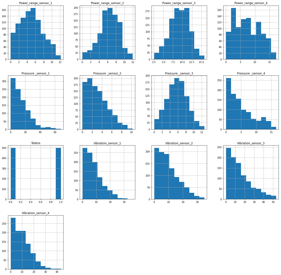
[外链图片转存失败,源站可能有防盗链机制,建议将图片保存下来直接上传(img-DynKjYBW-1576910854913)(output_10_1.png)]
# 定义要绘制两两关系的属性列
import seaborn as sns
numerical = [ u'Status',u'Power_range_sensor_2',u'Power_range_sensor_1','Power_range_sensor_4']
# 绘制关系图
g = sns.pairplot(test[numerical], hue='Status', palette='seismic', diag_kind = 'kde',diag_kws=dict(shade=True))
g.set(xticklabels=[])
<seaborn.axisgrid.PairGrid at 0x28d6004d1d0>
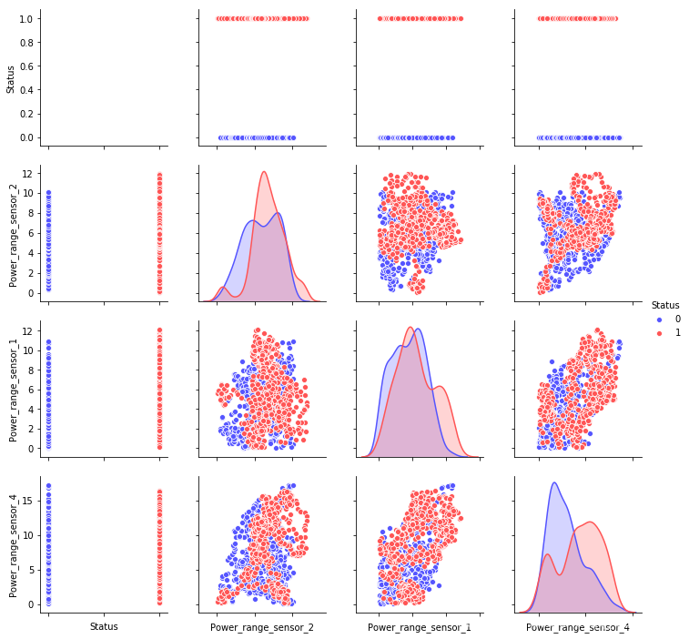
[外链图片转存失败,源站可能有防盗链机制,建议将图片保存下来直接上传(img-aZ65aejU-1576910854915)(output_11_1.png)]
import seaborn as sns
sns.catplot(x='Status',y='Vibration_sensor_1',hue='Status',kind='box',data=test)
<seaborn.axisgrid.FacetGrid at 0x28d60b7acc0>
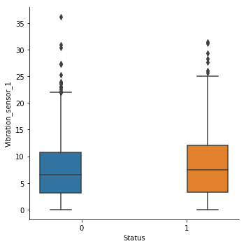
[外链图片转存失败,源站可能有防盗链机制,建议将图片保存下来直接上传(img-ooeJyiO1-1576910854917)(output_12_1.png)]
test['Vibration_sensor_2'].dropna().plot(kind='kde', xlim=(-50,100))
<matplotlib.axes._subplots.AxesSubplot at 0x28d60df1d68>
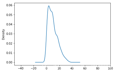
[外链图片转存失败,源站可能有防盗链机制,建议将图片保存下来直接上传(img-J6AvX6p8-1576910854918)(output_13_1.png)]
异常值
test_1=test.loc[test['Status']==1]
for i in test.columns:
    print(i)
    sns.catplot(y=i,kind='box',data=test_1)
Status
Power_range_sensor_1
Power_range_sensor_2
Power_range_sensor_3
Power_range_sensor_4
Pressure _sensor_1
Pressure _sensor_2
Pressure _sensor_3
Pressure _sensor_4
Vibration_sensor_1
Vibration_sensor_2
Vibration_sensor_3
Vibration_sensor_4
# Power_range_sensor_2<2,Pressure _sensor_1>40,Vibration_sensor_1>25,Vibration_sensor_2>30,Vibration_sensor_4>32,
test_1['Power_range_sensor_2'].ix[test_1['Power_range_sensor_2']<2] = 2
test_1['Pressure _sensor_1'].ix[test_1['Pressure _sensor_1']>40] = 40
test_1['Vibration_sensor_1'].ix[test_1['Vibration_sensor_1']>25] = 25
test_1['Vibration_sensor_2'].ix[test_1['Vibration_sensor_2']>30] = 30
test_1['Vibration_sensor_4'].ix[test_1['Vibration_sensor_4']>32] = 32
test_2=test.loc[test['Status']==0]
for i in test.columns:
    print(i)
    sns.catplot(y=i,kind='box',data=test_2)
Status
Power_range_sensor_1
Power_range_sensor_2
Power_range_sensor_3
Power_range_sensor_4
Pressure _sensor_1
Pressure _sensor_2
Pressure _sensor_3
Pressure _sensor_4
Vibration_sensor_1
Vibration_sensor_2
Vibration_sensor_3
Vibration_sensor_4
# Power_range_sensor_4>16,Pressure _sensor_1>42,Pressure _sensor_2>8,Pressure _sensor_4>13,Vibration_sensor_1>21,Vibration_sensor_2>32,Vibration_sensor_3>32,
test_2['Power_range_sensor_4'].ix[test_2['Power_range_sensor_4']>16] = 16
test_2['Pressure _sensor_1'].ix[test_2['Pressure _sensor_1']>42] = 42
test_2['Pressure _sensor_2'].ix[test_2['Pressure _sensor_2']>8] = 8
test_2['Pressure _sensor_4'].ix[test_2['Pressure _sensor_4']>13] = 13
test_2['Vibration_sensor_1'].ix[test_2['Vibration_sensor_1']>21] = 21
test_2['Vibration_sensor_2'].ix[test_2['Vibration_sensor_2']>32] = 32
test_2['Vibration_sensor_3'].ix[test_2['Vibration_sensor_3']>32] = 32
一座核电站正计划使用提供给你的数据集来训练分类器,以帮助核安全工程师监测和检测核反应堆是否正常工作。这将是非常有用的,因为这些参数是不断监测和储存的,因此可以用来分类不同反应堆的状态。一个机器学习实习生被要求在许多训练过的模型中选择性能最好的模型(例如,许多类型的分类器已经被训练过,如KNN, SVM,神经网络等)。实习生使用70%的数据作为训练集,20%的数据作为验证集,最后10%的数据作为测试集(通过选择可用特征的子集或使用不同类型的分类器),并记录测试集的准确性。实习生准确性达到90%认为这个模型是最好的。你会同意吗?为什么?请解释并详细说明
特征处理
from sklearn.preprocessing import StandardScaler
x = test.drop(['Status'],axis=1)
y=test['Status']
X_scaler = StandardScaler()
x = X_scaler.fit_transform(x)
print('data shape: {0}; no. positive: {1}; no. negative: {2}'.format(
    x.shape, y[y==1].shape[0], y[y==0].shape[0]))
from sklearn.model_selection import train_test_split
X_train, X_test, y_train, y_test = train_test_split(x, y, test_size=0.3)
data shape: (996, 12); no. positive: 498; no. negative: 498
print('data shape: {0}; no. positive: {1}; no. negative: {2}'.format(
    X_test.shape, y_test[y==1].shape[0], y_test[y==0].shape[0]))
from sklearn.model_selection import train_test_split
X_train2, X_test2, y_train2, y_test2 = train_test_split(X_test, y_test, test_size=0.1)
data shape: (299, 12); no. positive: 148; no. negative: 151
svm
from sklearn import svm
from sklearn.metrics import classification_report
svm = svm.SVC()
svm.fit(X_train, y_train)
print('----------------Train Set----------------------')
print(classification_report(y_train, svm.predict(X_train)))
print('----------------Validation set----------------------')
print(classification_report(y_test, svm.predict(X_test)))
print('----------------test set----------------------')
print(classification_report(y_test2, svm.predict(X_test2)))
----------------Train Set----------------------
             precision    recall  f1-score   support

          0       0.87      0.97      0.92       347
          1       0.97      0.86      0.91       350

avg / total       0.92      0.92      0.92       697

----------------Validation set----------------------
             precision    recall  f1-score   support

          0       0.87      0.91      0.89       151
          1       0.91      0.86      0.88       148

avg / total       0.89      0.89      0.89       299

----------------test set----------------------
             precision    recall  f1-score   support

          0       0.75      0.82      0.78        11
          1       0.89      0.84      0.86        19

avg / total       0.84      0.83      0.83        30
决策树模型
from sklearn.tree import DecisionTreeClassifier
tree = DecisionTreeClassifier()
tree.fit(X_train, y_train)
print('----------------Train Set----------------------')
print(classification_report(y_train, tree.predict(X_train)))
print('----------------Validation set----------------------')
print(classification_report(y_test, tree.predict(X_test)))
print('----------------test set----------------------')
print(classification_report(y_test2, tree.predict(X_test2)))
----------------Train Set----------------------
             precision    recall  f1-score   support

          0       1.00      1.00      1.00       347
          1       1.00      1.00      1.00       350

avg / total       1.00      1.00      1.00       697

----------------Validation set----------------------
             precision    recall  f1-score   support

          0       0.85      0.85      0.85       151
          1       0.85      0.85      0.85       148

avg / total       0.85      0.85      0.85       299

----------------test set----------------------
             precision    recall  f1-score   support

          0       0.69      0.82      0.75        11
          1       0.88      0.79      0.83        19

avg / total       0.81      0.80      0.80        30
构建LM神经网络模型
from keras.models import Sequential
from keras.layers.core import Dense,Activation
net_file='net.model'
net=Sequential()
net.add(Dense(input_dim=12,output_dim=10))
net.add(Activation('relu'))
net.add(Dense(input_dim=10,output_dim=1))
net.add(Activation('sigmoid'))
net.compile(loss='binary_crossentropy',optimizer='adam')
net.fit(X_train,y_train,nb_epoch=2,batch_size=10)
net.save_weights(net_file)
Using Theano backend.
WARNING (theano.configdefaults): g++ not available, if using conda: `conda install m2w64-toolchain`
D:\sofewore\anaconda\lib\site-packages\theano\configdefaults.py:560: UserWarning: DeprecationWarning: there is no c++ compiler.This is deprecated and with Theano 0.11 a c++ compiler will be mandatory
  warnings.warn("DeprecationWarning: there is no c++ compiler."
WARNING (theano.configdefaults): g++ not detected ! Theano will be unable to execute optimized C-implementations (for both CPU and GPU) and will default to Python implementations. Performance will be severely degraded. To remove this warning, set Theano flags cxx to an empty string.
WARNING (theano.tensor.blas): Using NumPy C-API based implementation for BLAS functions.
D:\sofewore\anaconda\lib\site-packages\ipykernel_launcher.py:5: UserWarning: Update your `Dense` call to the Keras 2 API: `Dense(input_dim=12, units=10)`
  """
D:\sofewore\anaconda\lib\site-packages\ipykernel_launcher.py:7: UserWarning: Update your `Dense` call to the Keras 2 API: `Dense(input_dim=10, units=1)`
  import sys
D:\sofewore\anaconda\lib\site-packages\ipykernel_launcher.py:10: UserWarning: The `nb_epoch` argument in `fit` has been renamed `epochs`.
  # Remove the CWD from sys.path while we load stuff.


Epoch 1/2
697/697 [==============================] - 2s 3ms/step - loss: 0.7389
Epoch 2/2
697/697 [==============================] - 2s 3ms/step - loss: 0.6885
print('----------------Train Set----------------------')
print(classification_report(y_train,net.predict_classes(X_train).reshape(len(X_train))))
print('----------------Validation set----------------------')
print(classification_report(y_test, net.predict_classes(X_test).reshape(len(X_test))))
print('----------------test set----------------------')
print(classification_report(y_test2,net.predict_classes(X_test2).reshape(len(X_test2))))
----------------Train Set----------------------
             precision    recall  f1-score   support

          0       0.60      0.56      0.58       347
          1       0.59      0.63      0.61       350

avg / total       0.60      0.60      0.60       697

----------------Validation set----------------------
             precision    recall  f1-score   support

          0       0.62      0.56      0.59       151
          1       0.59      0.65      0.62       148

avg / total       0.61      0.61      0.60       299

----------------test set----------------------
             precision    recall  f1-score   support

          0       0.43      0.55      0.48        11
          1       0.69      0.58      0.63        19

avg / total       0.59      0.57      0.57        30
朴素贝叶斯
from sklearn.naive_bayes import GaussianNB
model = GaussianNB()
model.fit(X_train, y_train)
print('----------------Train Set----------------------')
print(classification_report(y_train,model.predict(X_train)))
print('----------------Validation set----------------------')
print(classification_report(y_test, model.predict(X_test)))
print('----------------test set----------------------')
print(classification_report(y_test2,model.predict(X_test2)))
----------------Train Set----------------------
             precision    recall  f1-score   support

          0       0.71      0.80      0.75       347
          1       0.77      0.67      0.72       350

avg / total       0.74      0.74      0.74       697

----------------Validation set----------------------
             precision    recall  f1-score   support

          0       0.71      0.81      0.76       151
          1       0.78      0.66      0.71       148

avg / total       0.74      0.74      0.73       299

----------------test set----------------------
             precision    recall  f1-score   support

          0       0.54      0.64      0.58        11
          1       0.76      0.68      0.72        19

avg / total       0.68      0.67      0.67        30
KNN
from sklearn.neighbors import KNeighborsClassifier
knn = KNeighborsClassifier()
knn.fit(X_train, y_train)
print('----------------Train Set----------------------')
print(classification_report(y_train,knn.predict(X_train)))
print('----------------Validation set----------------------')
print(classification_report(y_test, knn.predict(X_test)))
print('----------------test set----------------------')
print(classification_report(y_test2,knn.predict(X_test2)))
----------------Train Set----------------------
             precision    recall  f1-score   support

          0       0.93      0.97      0.95       347
          1       0.97      0.92      0.95       350

avg / total       0.95      0.95      0.95       697

----------------Validation set----------------------
             precision    recall  f1-score   support

          0       0.90      0.87      0.89       151
          1       0.88      0.91      0.89       148

avg / total       0.89      0.89      0.89       299

----------------test set----------------------
             precision    recall  f1-score   support

          0       0.73      1.00      0.85        11
          1       1.00      0.79      0.88        19

avg / total       0.90      0.87      0.87        30
第三部分:算法设计(30%)
现在,您将设计一个人工神经网络(ANN)分类器,根据压水堆的基本工作条件,将其分类为正常或异常。您将使用提供的数据集来训练模型。设计神经网络时,使用具有两个隐层的全连通神经网络结构;隐层采用sigmoid函数作为非线性激活函数,输出层采用logistic函数;将隐藏层中的神经元数量设置为500。现在随机选择90%的数据作为训练集,作为测试集,其余10%。使用训练数据训练安,和计算的准确性,即分类的比例适当的情况下,使用测试集,请报告如何将数据分为训练集和测试集。另外,请详细汇报ANN的培训步骤,并给出准确性结果。
**好处:你可以尝试不同数量的epoch来监控随着算法的不断学习准确性如何变化,你可以使用x轴上的epoch数量和y轴上的准确性来绘制。
现在使用相同的训练和测试数据来训练一个随机森林分类器。设置a)树的数量=
1000和b)一个叶节点所需的最小样本数={5和50}。请报告随机森林的训练步骤,并显示测试集的准确性结果
**好处:你可以调整树的数量,并监控性能如何变化,因为更多的树被添加,例如10,50,100,1000,5000树,等等。
# coding:utf-8
import tensorflow as tf
from numpy.random import RandomState

# 使用命名空间定义元素,便于使用tensorboard查看神经网络图形化
with tf.name_scope('graph_1') as scope:
    batch_size = 697 # 神经网络训练集batch大小为500
    cell=500
    # 定义神经网络的结构,输入为2个参数,隐藏层为10个参数,输出为1个参数
    # w1为输入到隐藏层的权重,2*10的矩阵(2表示输入层有2个因子,也就是两列输入,10表示隐藏层有10个cell)
    w1 = tf.Variable(tf.random_normal([12, cell], stddev=1, seed=1), name='w1')
    # w2为隐藏层到输出的权重,10*1的矩阵(接受隐藏的10个cell输入,输出1列数据)
    w2 = tf.Variable(tf.random_normal([cell, 2], stddev=1, seed=1), name='w2')
    # b1和b2均为一行,列数对应由w1和w2的列数决定
    b1 = tf.Variable(tf.random_normal([1, cell], stddev=1, seed=1), name='b1')
    b2 = tf.Variable(tf.random_normal([1, 1], stddev=1, seed=1), name='b2')

    # 维度中使用None,则可以不规定矩阵的行数,方便存储不同batch的大小。(占位符)
    x = tf.placeholder(tf.float32, shape=(None,12), name='x-input')
    y_ = tf.placeholder(tf.float32, shape=(None,1), name='y-input')

    # 定义神经网络前向传播的过程,定义了1层隐藏层。
    # 输入到隐藏、隐藏到输出的算法均为逻辑回归,即y=wx+b的模式
    a = tf.add(tf.matmul(x, w1, name='a'), b1)
    y = tf.add(tf.matmul(tf.sigmoid(a), w2, name='y'), b2)  # 使用tanh激活函数使模型非线性化
    y_hat = tf.sigmoid(y)  # 将逻辑回归的输出概率化

    # 定义损失函数和反向传播的算法,见吴恩达视频课程第二周第三节课,逻辑回归的损失函数
    cross_entropy = - \
        tf.reduce_mean(y_ * tf.log(tf.clip_by_value(y_hat, 1e-10, 1.0)) +
                       (1-y_)*tf.log(tf.clip_by_value((1-y_hat), 1e-10, 1.0)))
    # 方差损失函数,逻辑回归不能用
    # cost = -tf.reduce_mean(tf.square(y_ - y_hat))
    # clip_by_value函数将y限制在1e-10和1.0的范围内,防止出现log0的错误,即防止梯度消失或爆发

    train_step = tf.train.AdamOptimizer(0.0001).minimize((cross_entropy))  # 反向传播算法
    dataset_size=697
    X=X_train
    Y = [[i] for i in y_train]
num=[]
cost_accum=[]
# 创建会话
with tf.Session() as sess:
    writer = tf.summary.FileWriter("logs/", sess.graph)
    init_op = tf.global_variables_initializer()  # 所有需要初始化的值
    sess.run(init_op)  # 初始化变量
#     print(sess.run(w1))
#     print(sess.run(w2))
#     print('x_hat =', x_hat, 'y_hat =', sess.run(y_hat, feed_dict={x: x_hat}))

    '''
    # 在训练之前神经网络权重的值,w1,w2,b1,b2的值
    '''

    # 设定训练的轮数
    STEPS = 10000
    for i in range(STEPS):
        # 每次从数据集中选batch_size个数据进行训练
        start = (i * batch_size) % dataset_size  # 训练集在数据集中的开始位置
        # 结束位置,若超过dataset_size,则设为dataset_size
        end = min(start + batch_size, dataset_size)

        # 通过选取的样本训练神经网络并更新参数
        sess.run(train_step, feed_dict={x: X[start:end], y_: Y[start:end]})
        if i % 1000 == 0:
            # 每隔一段时间计算在所有数据上的损失函数并输出
            total_cross_entropy = sess.run(
                cross_entropy, feed_dict={x: X, y_: Y})
            total_w1 = sess.run(w1)
            total_b1 = sess.run(b1)
            total_w2 = sess.run(w2)
            total_b2 = sess.run(b2)
            print("After %d training steps(s), cross entropy on all data is %g" % (
                i, total_cross_entropy))
            num.append(i)
            cost_accum.append(total_cross_entropy)
#             print('w1=', total_w1, ',b1=', total_b1)
#             print('w2=', total_w2, ',b2=', total_b2)

    # 在训练之后神经网络权重的值
#     print(sess.run(w1))
#     print(sess.run(w2))
#     print('x_hat =', x_hat, 'y_hat =', sess.run(y_hat, feed_dict={x: x_hat}))
WARNING:tensorflow:From D:\sofewore\anaconda\lib\site-packages\tensorflow_core\python\ops\math_grad.py:1424: where (from tensorflow.python.ops.array_ops) is deprecated and will be removed in a future version.
Instructions for updating:
Use tf.where in 2.0, which has the same broadcast rule as np.where
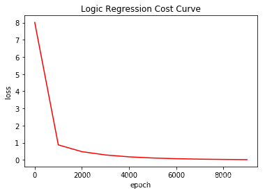
After 0 training steps(s), cross entropy on all data is 8.0108
After 1000 training steps(s), cross entropy on all data is 0.87692
After 2000 training steps(s), cross entropy on all data is 0.482967
After 3000 training steps(s), cross entropy on all data is 0.290985
After 4000 training steps(s), cross entropy on all data is 0.179876
After 5000 training steps(s), cross entropy on all data is 0.113813
After 6000 training steps(s), cross entropy on all data is 0.0728121
After 7000 training steps(s), cross entropy on all data is 0.0465708
After 8000 training steps(s), cross entropy on all data is 0.0295726
After 9000 training steps(s), cross entropy on all data is 0.0185979
plt.plot(num,cost_accum,'r')
plt.title('Logic Regression Cost Curve')
plt.xlabel('epoch')
plt.ylabel('loss')
plt.show()
from sklearn.ensemble import RandomForestClassifier
from sklearn.naive_bayes import GaussianNB
# 构建GaussianNB模型(默认参数即可),并调用fit进行模型拟合
min_samples_leaf=[5,50]
for i in min_samples_leaf:
    sjsl = RandomForestClassifier(min_samples_leaf=i,n_estimators=100)
    sjsl.fit(X_train, y_train)
    print('----------------test set n_estimators=100,min_samples_leaf={0}----------------------'.format(i))
    print(classification_report(y_test2,sjsl.predict(X_test2)))
#n_estimators=100 树的数量
#min_samples_leaf=5,50
D:\sofewore\anaconda\lib\site-packages\sklearn\ensemble\weight_boosting.py:29: DeprecationWarning: numpy.core.umath_tests is an internal NumPy module and should not be imported. It will be removed in a future NumPy release.
  from numpy.core.umath_tests import inner1d


----------------test set n_estimators=100,min_samples_leaf=5----------------------
             precision    recall  f1-score   support

          0       0.75      0.82      0.78        11
          1       0.89      0.84      0.86        19

avg / total       0.84      0.83      0.83        30

----------------test set n_estimators=100,min_samples_leaf=50----------------------
             precision    recall  f1-score   support

          0       0.64      0.64      0.64        11
          1       0.79      0.79      0.79        19

avg / total       0.73      0.73      0.73        30
第四部分:
模型选择(20%)
你已经设计了几乎固定模型参数的ANN和随机森林分类器。当这些模型参数改变时,模型的性能可能会发生变化。您希望了解哪一组参数是更可取的,并在给定选项范围的情况下选择最佳参数集。为此,一种方法是采用交叉验证(CV)过程。在这个任务中,你需要使用一份10倍的简历。作为第一步,将数据随机分成10个几乎相同大小的倍数,并报告为此所采取的步骤。
对于ANN,将隐含层的神经元数量设置为50,500和1000。对于随机森林,将树的数量设置为20,500和10000,并在您选择的叶节点上设置所需的最小样本数量(如果您选择使用预先构建的库而不自己开发它,则设置为默认值;两种方法都可以报告这个值)。
两种方法请分别完成以下任务:a)使用10倍CV法分别为ANN和random forest选择最佳的神经元数目或树数。b)报告将CV应用到每个组合/模型的过程。c)报告每组参数的平均精度结果,即对应不同数量的神经元和不同数量的树。对于这两种方法,我们分别应该使用哪些参数,即ANN和random forest
到目前为止,您已经为每个方法选择了最好的参数,但是我们还没有决定哪个模型是最好的。根据目前的结果,对于这个数据集,在所有的ANNs和随机森林的组合中,哪一个是最好的模型?请讨论和证明你的选择,反映你的知识到目前为止。
from sklearn.model_selection import GridSearchCV
n_estimatorss=[20,500,10000]
# Set the parameters by cross-validation
param_grid = {'n_estimators': n_estimatorss}
clf = GridSearchCV(RandomForestClassifier(), param_grid, cv=10, return_train_score=True)
clf.fit(X_train,y_train)
print("best param: {0}\nbest score: {1}".format(clf.best_params_,
                                                clf.best_score_))
best param: {'n_estimators': 10000}
best score: 0.9024390243902439
# import keras
# from keras.wrappers.scikit_learn import KerasClassifier
# from sklearn.model_selection import cross_val_score
# from keras.models import Sequential
# from keras.layers import Dense
# for i in [50,500,1000]:
#     classifier = Sequential()
#     classiifier.add(Dense(i,kernel_initializer = 'uniform', activation = 'relu', input_dim=12))
#     classifier.add(Dense(1, kernel_initializer = 'uniform', activation = 'sigmoid'))
#     classifier.compile(optimizer= 'adam',loss = 'binary_crossentropy',metrics = ['accuracy'])
#     classifier.fit(X_train, y_train, batch_size = 100, epochs = 300)
#     print(' nerve cell{} accuracy rate '.format(i))
import keras
from keras.models import Sequential
from keras.layers import Dense
classifier = Sequential()
for i in [50,500,1000]:
    classifier = Sequential()
    classifier.add(Dense(i, kernel_initializer = 'uniform',activation ='sigmoid', input_dim=12))
    classifier.add(Dense(1, kernel_initializer = 'uniform',activation ='sigmoid'))
    classifier.compile(optimizer= 'adam',loss = 'binary_crossentropy',metrics = ['accuracy'])
    classifier.fit(X_train, y_train, batch_size = 700, epochs = 1)
    print(' nerve cell{} accuracy rate '.format(i))


 655
655


 被折叠的 条评论
为什么被折叠?
被折叠的 条评论
为什么被折叠?
 到【灌水乐园】发言


