机器学习：逻辑回归

目录

一、理论知识

1、Sigmoid激活函数

2、逻辑回归模型

3、损失函数（交叉熵损失）

4、梯度计算

5、梯度下降

二、代码实现

1、导入Python包

2、利用sklearn构造二分类数据集

3、定义sigmoid激活函数

4、定义前向传播函数、损失函数、反向传播函数

5、定义并初始化权重参数 W 和 b

6、划分训练集和测试集

7、模型训练

8、模型测试 

---

一、理论知识

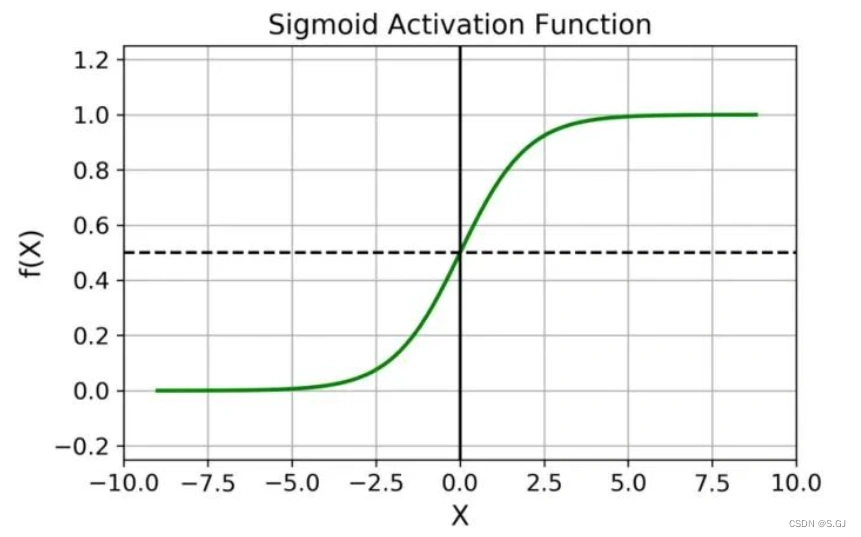
1、Sigmoid激活函数

Sigmoid激活函数将实数输入映射到(0, 1)区间，可用于二分类任务，其数学定义如下：

其函数图像为：

其导数为：

 

2、逻辑回归模型

其中，表示输入，表示输出，和表示可学习的权重参数，表示Sigmoid激活函数。逻辑回归模型与线性回归模型的区别在于逻辑回归模型多了一个激活函数。

3、损失函数（交叉熵损失）

其中，，。当时，，损失达到最小。同样地，当时，，损失达到最小。

4、梯度计算

注：梯度计算的结果与线性回归模型的结果一致。

5、梯度下降

其中，是梯度下降步长，又称学习率。多次迭代执行前向传播（计算映射函数）和反向传播（梯度计算+梯度下降），损失函数最终收敛至局部最优解。

二、代码实现

1、导入Python包

import numpy as np
import matplotlib.pyplot as plt
from sklearn.datasets import make_blobs
from sklearn.model_selection import train_test_split
 
plt.rcParams['font.sans-serif'] = ['Times New Roman']

2、利用sklearn构造二分类数据集

data, target = make_blobs(n_samples=1000, n_features=2, centers=2, random_state=2024)

plt.figure(dpi=100)
plt.scatter(data[:,0], data[:,1], c=target)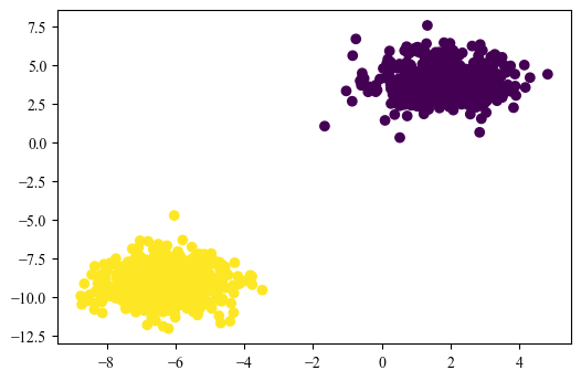

3、定义sigmoid激活函数

def sigmoid(z):
    return 1/(1+np.exp(-z))

4、定义前向传播函数、损失函数、反向传播函数

def forward(X, weights, bias):
    Y_hat = sigmoid(np.dot(X, weights) + bias)
    return Y_hat

def Loss_fuction(Y, Y_hat):
    N = Y.shape[0]
    cost = -1 / N * np.sum(Y * np.log(Y_hat) + (1 - Y) * np.log(1 - Y_hat))
    return cost

def backward(X, Y, Y_hat, weights, bias, lr):
    # 梯度计算
    N = Y.shape[0]
    dw = 1 / N * np.dot(X.T, (Y_hat - Y))
    db = 1 / N * np.sum(Y_hat - Y)

    # 权重更新
    weights -= lr * dw
    bias -= lr * db
    return weights, bias

5、定义并初始化权重参数 W 和 b

weights = np.zeros((2, 1))
bias = 0

6、划分训练集和测试集

X = data
Y = target[:,None]
X_train, X_test, Y_train, Y_test = train_test_split(X, Y, test_size=0.2, random_state=2024)
print(X_train.shape, X_test.shape, Y_train.shape, Y_test.shape)

7、模型训练

lr = 0.01 # 学习率
epochs = 1000  # 迭代次数
train_loss = []
for _ in range(epochs):
    # 前向传播
    Y_hat = forward(X_train, weights, bias)
 
    # 损失计算
    loss = Loss_fuction(Y_train, Y_hat)
    train_loss.append(loss)
 
    # 反向传播
    weights, bias = backward(X_train, Y_train, Y_hat, weights, bias, lr)

plt.figure(dpi=100)
plt.plot(train_loss)
plt.xlabel("Epoch")
plt.ylabel("Loss")
plt.title("Training Loss")
plt.show()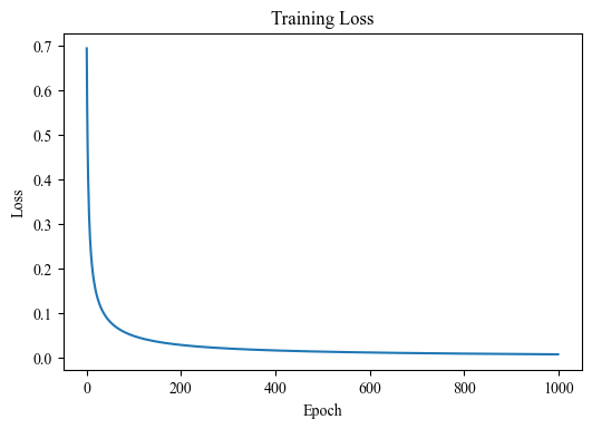

8、模型测试 

threshold = 0.5  # 判断正负类的阈值

y_predict = forward(X_test, weights, bias)
print(f"Test ACC: {np.mean((y_predict>threshold) == Y_test)}")

Test ACC: 1.0