wandb: 深度学习轻量级可视化工具入门教程

本文，就来给大家介绍一款新型的机器学习可视化工具，能够让人工智能研发过程变得更加简单明了。

引言

人工智能方向的项目，和数据可视化是紧密相连的。

模型训练过程中梯度下降过程是什么样的？损失函数的走向如何？训练模型的准确度怎么变化的？

清楚这些数据，对我们模型的优化至关重要。

由于人工智能项目往往伴随着巨大数据量，用肉眼去逐个数据查看、分析是不显示的。这时候就需要用到数据可视化和日志分析报告。

TensorFlow自带的Tensorboard在模型和训练过程可视化方面做得越来越好。但是，也越来越臃肿，对于初入人工智能的同学来说有一定的门槛。

人工智能方面的项目变得越来越规范化，以模型训练、数据集准备为例，目前很多大公司已经发布了各自的自动机器学习平台，让工程师把更多精力放在优化策略上，而不是在准备数据、数据可视化方面。

wandb

wandb是Weights & Biases的缩写，这款工具能够帮助跟踪你的机器学习项目。它能够自动记录模型训练过程中的超参数和输出指标，然后可视化和比较结果，并快速与同事共享结果。

通过wandb，能够给你的机器学习项目带来强大的交互式可视化调试体验，能够自动化记录Python脚本中的图标，并且实时在网页仪表盘展示它的结果，例如，损失函数、准确率、召回率，它能够让你在最短的时间内完成机器学习项目可视化图片的制作。

总结而言，wandb有4项核心功能：

• 看板：跟踪训练过程，给出可视化结果
• 报告：保存和共享训练过程中一些细节、有价值的信息
• 调优：使用超参数调优来优化你训练的模型
• 工具：数据集和模型版本化

也就是说，wandb并不单纯的是一款数据可视化工具。它具有更为强大的模型和数据版本管理。此外，还可以对你训练的模型进行调优。

wandb另外一大亮点的就是强大的兼容性，它能够和Jupyter、TensorFlow、Pytorch、Keras、Scikit、fast.ai、LightGBM、XGBoost一起结合使用。

因此，它不仅可以给你带来时间和精力上的节省，还能够给你的结果带来质的改变。

验证数据可视化

wandb会自动选取一部分验证数据，然后把它展示到面板上。例如，手写体预测的结果、目标识别的包围盒。

自然语言处理

使用自定义图表可视化基于NLP注意力的模型

这里只给出2个示例，除了这些，它目前还有更多实用有价值的功能。而且，它还不断在增加新功能。

重要工具

wandb(Weights & Biases)是一个类似于tensorboard的极度丝滑的在线模型训练可视化工具。

wandb这个库可以帮助我们跟踪实验，记录运行中的超参数和输出指标，可视化结果并共享结果。

下图展示了wandb这个库的功能，Framework Agnostic的意思是无所谓你用什么框架，均可使用wandb。wandb可与用户的机器学习基础架构配合使用：AWS，GCP，Kubernetes，Azure和本地机器。

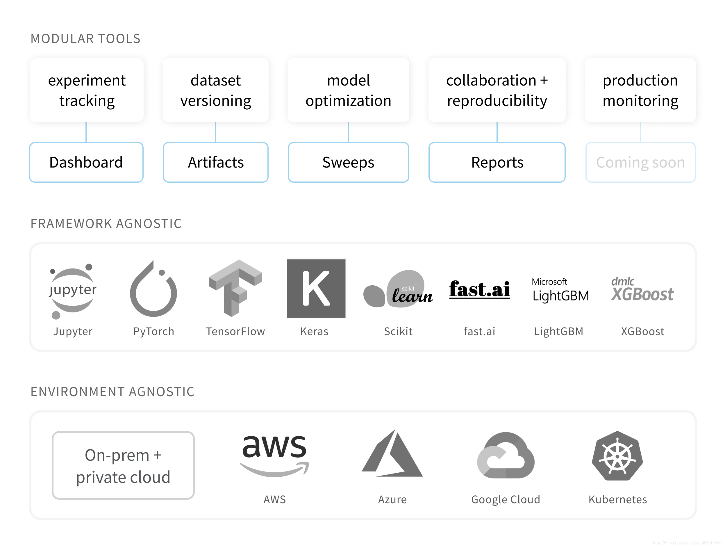
下面是wandb的重要的工具

• Dashboard: Track experiments（跟踪实验）, visualize results（可视化结果）；
• Reports：Save and share reproducible findings（分享和保存结果）；
• Sweeps：Optimize models with hyperparameter tuning（超参调优）；
• Artifacts：Dataset and model versioning, pipeline tracking（数据集和模型的版本控制）；

极简教程

1 安装库

pip install wandb

2 创建账户

wandb login

3 初始化

# Inside my model training code
import wandb
wandb.init(project="my-project")

4 声明超参数

wandb.config.dropout = 0.2
wandb.config.hidden_layer_size = 128

5 记录日志

def my_train_loop():
    for epoch in range(10):
        loss = 0 # change as appropriate :)
        wandb.log({'epoch': epoch, 'loss': loss})

6 保存文件

# by default, this will save to a new subfolder for files associated
# with your run, created in wandb.run.dir (which is ./wandb by default)
wandb.save("mymodel.h5")

# you can pass the full path to the Keras model API
model.save(os.path.join(wandb.run.dir, "mymodel.h5"))

使用wandb以后，模型输出，log和要保存的文件将会同步到cloud。

PyTorch应用wandb

我们以一个最简单的神经网络为例展示wandb的用法：

首先导入必要的库：

from __future__ import print_function
import argparse
import random  # to set the python random seed
import numpy  # to set the numpy random seed
import torch
import torch.nn as nn
import torch.nn.functional as F
import torch.optim as optim
from torchvision import datasets, transforms
from torch.utils.data import DataLoader
# Ignore excessive warnings
import logging

logging.propagate = False
logging.getLogger().setLevel(logging.ERROR)

# WandB – Import the wandb library
import wandb

登陆你的wandb账户：

# WandB – Login to your wandb account so you can log all your metrics
!wandb login

定义Convolutional Neural Network：

# 定义Convolutional Neural Network：

class Net(nn.Module):
    def __init__(self):
        super(Net, self).__init__()

        # In our constructor, we define our neural network architecture that we'll use in the forward pass.
        # Conv2d() adds a convolution layer that generates 2 dimensional feature maps
        # to learn different aspects of our image.
        self.conv1 = nn.Conv2d(3, 6, kernel_size=5)
        self.conv2 = nn.Conv2d(6, 16, kernel_size=5)

        # Linear(x,y) creates dense, fully connected layers with x inputs and y outputs.
        # Linear layers simply output the dot product of our inputs and weights.
        self.fc1 = nn.Linear(16 * 5 * 5, 120)
        self.fc2 = nn.Linear(120, 84)
        self.fc3 = nn.Linear(84, 10)

    def forward(self, x):
        # Here we feed the feature maps from the convolutional layers into a max_pool2d layer.
        # The max_pool2d layer reduces the size of the image representation our convolutional layers learnt,
        # and in doing so it reduces the number of parameters and computations the network needs to perform.
        # Finally we apply the relu activation function which gives us max(0, max_pool2d_output)
        x = F.relu(F.max_pool2d(self.conv1(x), 2))
        x = F.relu(F.max_pool2d(self.conv2(x), 2))

        # Reshapes x into size (-1, 16 * 5 * 5)
        # so we can feed the convolution layer outputs into our fully connected layer.
        x = x.view(-1, 16 * 5 * 5)

        # We apply the relu activation function and dropout to the output of our fully connected layers.
        x = F.relu(self.fc1(x))
        x = F.relu(self.fc2(x))
        x = self.fc3(x)

        # Finally we apply the softmax function to squash the probabilities of each class (0-9)
        # and ensure they add to 1.
        return F.log_softmax(x, dim=1)

定义训练函数

def train(config, model, device, train_loader, optimizer, epoch):
    # switch model to training mode. This is necessary for layers like dropout, batchNorm etc.
    # which behave differently in training and evaluation mode.
    model.train()

    # we loop over the data iterator, and feed the inputs to the network and adjust the weights.
    for batch_id, (data, target) in enumerate(train_loader):
        if batch_id > 20:
            break
        # Loop the input features and labels from the training dataset.
        data, target = data.to(device), target.to(device)

        # Reset the gradients to 0 for all learnable weight parameters
        optimizer.zero_grad()

        # Forward pass: Pass image data from training dataset, make predictions
        # about class image belongs to (0-9 in this case).
        output = model(data)

        # Define our loss function, and compute the loss
        loss = F.nll_loss(output, target)

        # Backward pass:compute the gradients of loss,the model's parameters
        loss.backward()

        # update the neural network weights
        optimizer.step()

定义测试函数

# wandb.log用来记录一些日志(accuracy,loss and epoch), 便于随时查看网路的性能
def test(args, model, device, test_loader, classes):
    model.eval()
    # switch model to evaluation mode.
    # This is necessary for layers like dropout, batchNorm etc. which behave differently in training and evaluation mode
    test_loss = 0
    correct = 0
    example_images = []

    with torch.no_grad():
        for data, target in test_loader:
            # Load the input features and labels from the test dataset
            data, target = data.to(device), target.to(device)

            # Make predictions: Pass image data from test dataset,
            # make predictions about class image belongs to(0-9 in this case)
            output = model(data)

            # Compute the loss sum up batch loss
            test_loss += F.nll_loss(output, target, reduction='sum').item()

            # Get the index of the max log-probability
            pred = output.max(1, keepdim=True)[1]
            correct += pred.eq(target.view_as(pred)).sum().item()

            # Log images in your test dataset automatically,
            # along with predicted and true labels by passing pytorch tensors with image data into wandb.
            example_images.append(wandb.Image(
                data[0], caption="Pred:{} Truth:{}".format(classes[pred[0].item()], classes[target[0]])))

   # wandb.log(a_dict) logs the keys and values of the dictionary passed in and associates the values with a step.
   # You can log anything by passing it to wandb.log(),
   # including histograms, custom matplotlib objects, images, video, text, tables, html, pointclounds and other 3D objects.
   # Here we use it to log test accuracy, loss and some test images (along with their true and predicted labels).
    wandb.log({
        "Examples": example_images,
        "Test Accuracy": 100. * correct / len(test_loader.dataset),
        "Test Loss": test_loss
    })

初始化一个wandb run，并设置超参数：

# 初始化一个wandb run, 并设置超参数
# Initialize a new run
wandb.init(project="pytorch-intro")
wandb.watch_called = False  # Re-run the model without restarting the runtime, unnecessary after our next release

# config is a variable that holds and saves hyper parameters and inputs
config = wandb.config  # Initialize config
config.batch_size = 4  # input batch size for training (default:64)
config.test_batch_size = 10  # input batch size for testing(default:1000)
config.epochs = 50  # number of epochs to train(default:10)
config.lr = 0.1  # learning rate(default:0.01)
config.momentum = 0.1  # SGD momentum(default:0.5)
config.no_cuda = False  # disables CUDA training
config.seed = 42  # random seed(default:42)
config.log_interval = 10  # how many batches to wait before logging training status

主函数

def main():
    use_cuda = not config.no_cuda and torch.cuda.is_available()
    device = torch.device("cuda:0" if use_cuda else "cpu")
    kwargs = {'num_workers': 1, 'pin_memory': True} if use_cuda else {}

    # Set random seeds and deterministic pytorch for reproducibility
    # random.seed(config.seed)      # python random seed
    torch.manual_seed(config.seed)  # pytorch random seed
    # numpy.random.seed(config.seed) # numpy random seed
    torch.backends.cudnn.deterministic = True

    # Load the dataset: We're training our CNN on CIFAR10.
    # First we define the transformations to apply to our images.
    transform = transforms.Compose([
        transforms.ToTensor(),
        transforms.Normalize((0.5, 0.5, 0.5), (0.5, 0.5, 0.5))
    ])

    # Now we load our training and test datasets and apply the transformations defined above
    train_loader = DataLoader(datasets.CIFAR10(
        root='./data',
        train=True,
        download=True,
        transform=transform
    ), batch_size=config.batch_size, shuffle=True, **kwargs)

    test_loader = DataLoader(datasets.CIFAR10(
        root='./data',
        train=False,
        download=True,
        transform=transform
    ), batch_size=config.batch_size, shuffle=False, **kwargs)

    classes = ('plane', 'car', 'bird', 'cat', 'deer', 'dog', 'frog', 'horse', 'ship', 'truck')
    # Initialize our model, recursively go over all modules and convert their parameters
    # and buffers to CUDA tensors (if device is set to cuda)
    model = Net().to(device)
    optimizer = optim.SGD(model.parameters(), lr=config.lr, momentum=config.momentum)

    # wandb.watch() automatically fetches all layer dimensions, gradients, model parameters
    # and logs them automatically to your dashboard.
    # using log="all" log histograms of parameter values in addition to gradients
    wandb.watch(model, log="all")
    for epoch in range(1, config.epochs + 1):
        train(config, model, device, train_loader, optimizer, epoch)
        test(config, model, device, test_loader, classes)

    # Save the model checkpoint. This automatically saves a file to the cloud
    torch.save(model.state_dict(), 'model.h5')
    wandb.save('model.h5')


if __name__ == '__main__':
    main()

参考文献

1. https://www.jianshu.com/p/148c108b00f0
2. https://zhuanlan.zhihu.com/p/266337608