


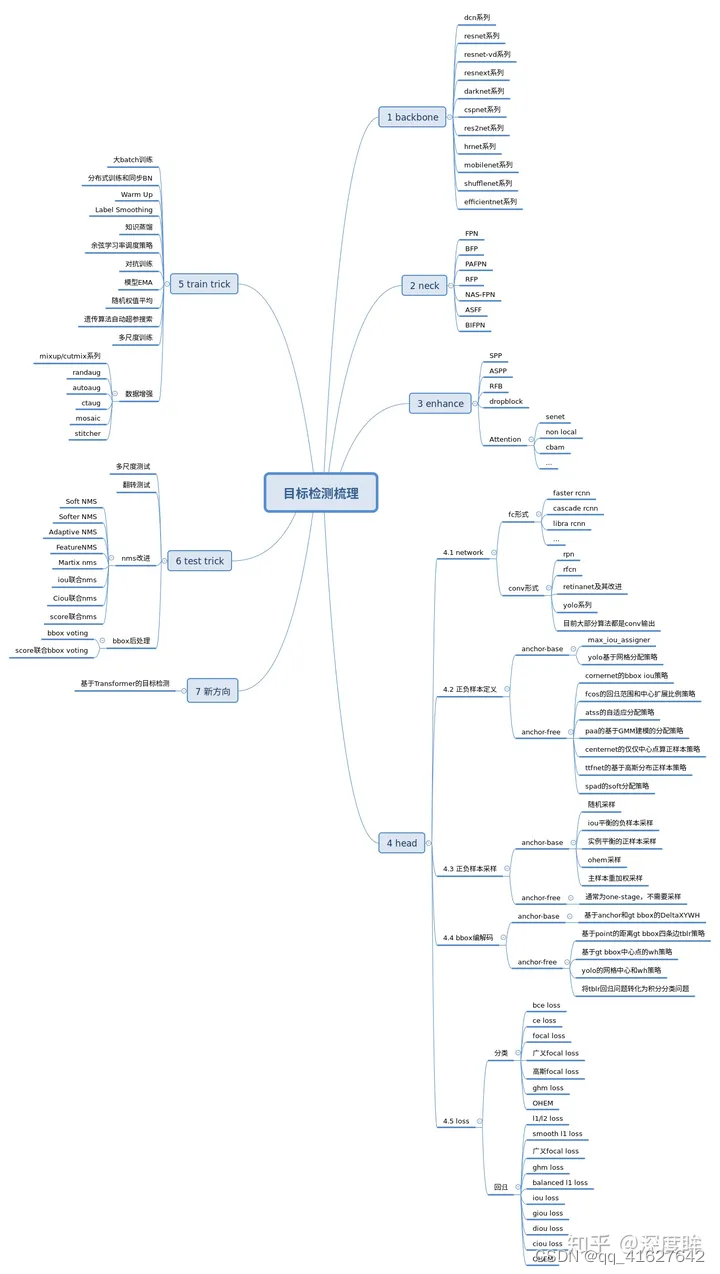
(一)、MMDetection 学习和进阶路线(一)
1、不得不知的 MMDetection 学习路线(个人经验版)
2、轻松掌握 MMDetection 整体构建流程(一)
3、轻松掌握 MMDetection 整体构建流程(二)
4、轻松掌握 MMDetection 中 Head 流程
5、MMCV 核心组件分析(四): Config
6、MMCV 核心组件分析(五): Registry
7、MMCV 核心组件分析(六): Hook
8、MMCV 核心组件分析(七): Runner
9、PyTorch 源码解读系列
10、 mmdetection的configs中的各项参数具体解释
11、轻松掌握 MMDetection 中常用算法(一):RetinaNet 及配置详解
12、 轻松掌握 MMDetection 中常用算法(二):Faster R-CNN|Mask R-CNN
13、 轻松掌握 MMDetection 中常用算法(三):FCOS
轻松掌握 MMDetection 中常用算法(四):ATSS
轻松掌握 MMDetection 中常用算法(五):Cascade R-CNN
轻松掌握 MMDetection 中常用算法(六):YOLOF
轻松掌握 MMDetection 中常用算法(七):CenterNet
轻松掌握 MMDetection 中常用算法(八):YOLACT
轻松掌握 MMDetection 中常用算法(九):AutoAssign
mmdetection最小复刻版(一):整体概览
mmdetection最小复刻版(二):RetinaNet和YoloV3分析
mmdetection源码笔记(二):模型之registry.py和builder.py解读(上)
mmdetection源码笔记(一):train.py解读
OpenMMLab 进阶指南,模型训练测试全流程解析
小白都能看懂!手把手教你使用混淆矩阵分析目标检测
以动制动 | Transformer 如何处理动态输入尺寸
OpenMMLab Playground:社区共探 SAM
DINOv2:无需微调,填补 SAM 的空白,支持多个下游任务
(二)、目标检测比赛中的tricks
1、 写给新手炼丹师:2021版调参上分手册
2、 目标检测比赛中的tricks(已更新更多代码解析)
3、 DOTAv2遥感图像旋转目标检测竞赛经验分享(Swin Transformer + Anchor free/based方案)
4、 华为云杯”2020深圳开放数据应用创新大赛·生活垃圾图片分类(目标检测)
5、图像分类比赛tricks:“观云识天”人机对抗大赛:机器图像算法赛道-天气识别—百万奖金
6、 图像分类比赛tricks:华为云人工智能大赛·垃圾分类挑战杯
7、水下目标检测算法赛解决方案分享 | 2020年全国水下机器人(湛江)大赛 -
8、 目标检测比赛笔记
9、 大比分领先!ACCV 2022 大规模细粒度图像分类冠军方案
(三)数据可视化并分析anchor_ratio设置等问题
1、 数据的简单分析和可视
2、 目标检测数据可视化,分析anchor_ratio的设置问题
3、 mmdetection 代码库中的 anchor 设置原则
4、基于mmdetection框架算法可视化分析随笔(上)
5、mmdetection最小复刻版(三):数据分析神兵利器
6、mmdetection最小复刻版(七):anchor-base和anchor-free差异分析
(四)数据增强
1、 一段代码玩转数据增强的N种方法
2、 MMClassification 数据增强介绍(二)
3、MMDetection 支持数据增强神器 Simple Copy Paste 全过程
4、目标检测tricks:Ablu数据库增强
5、图像分类训练技巧之数据增强篇
6、12种常用图像数据增强技术总结
(五)Multi-scale Training/Testing 多尺度训练/测试
1、 目标检测比赛中的tricks(已更新更多代码解析)
2、水下目标检测算法赛解决方案分享 | 2020年全国水下机器人(湛江)大赛 -
3、 MMDetection 图像缩放 Resize 详细说明
4、Crowdhuman人体检测比赛第一名经验总结
5、使用多尺度策略来训练 Mask R-CNN
一些中间变量在配置文件中使用,例如数据集中的train_pipeline/ test_pipeline。值得注意的是,当修改子配置中的中间变量时,用户需要再次将中间变量传递到相应的字段中。例如,我们想使用多尺度策略来训练 Mask R-CNN。train_pipeline/test_pipeline是我们要修改的中间变量。
_base_ = './mask-rcnn_r50_fpn_1x_coco.py'

train_pipeline = [
    dict(type='LoadImageFromFile'),
    dict(type='LoadAnnotations', with_bbox=True, with_mask=True),
    dict(
        type='RandomResize', scale=[(1333, 640), (1333, 800)],
        keep_ratio=True),
    dict(type='RandomFlip', prob=0.5),
    dict(type='PackDetInputs')
]
test_pipeline = [
    dict(type='LoadImageFromFile'),
    dict(type='Resize', scale=(1333, 800), keep_ratio=True),
    dict(
        type='PackDetInputs',
        meta_keys=('img_id', 'img_path', 'ori_shape', 'img_shape',
                   'scale_factor'))
]
train_dataloader = dict(dataset=dict(pipeline=train_pipeline))
val_dataloader = dict(dataset=dict(pipeline=test_pipeline))
test_dataloader = dict(dataset=dict(pipeline=test_pipeline))
我们首先定义新的train_pipeline/test_pipeline并将它们传递到数据加载器字段中。
(六)学习率和batchsize的关系、学习率自动缩放
深度学习中学习率和batchsize对模型准确率的影响
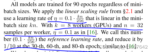
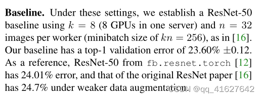
学习率自动缩放
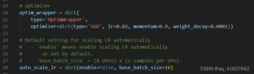
重要提示:配置文件中的默认学习率适用于 8 个 GPU,每个 GPU 2 个样本(批量大小 = 8 * 2 = 16)。它已被设置为auto_scale_lr.base_batch_size in config/base/schedules/schedule_1x.py。当批量大小为 16时,学习率将根据该值自动缩放。同时,为了不影响其他基于mmdet的代码库,该标志默认auto_scale_lr.enable设置为False。
如果要启用此功能,则需要添加 argument --auto-scale-lr。在处理命令之前,您需要检查要使用的配置名称,因为配置名称表示默认的批量大小。默认, it is 8 x 2 = 16 batch size, like faster_rcnn_r50_caffe_fpn_90k_coco.py or pisa_faster_rcnn_x101_32x4d_fpn_1x_coco.py。在其他情况下,您将看到配置文件名中包含_NxM_,like cornernet_hourglass104_mstest_32x3_210e_coco.py which batch size is 32 x 3 = 96, or scnet_x101_64x4d_fpn_8x1_20e_coco.py which batch size is 8 x 1 = 8。
he basic usage of learning rate auto scaling is as follows.
python tools/train.py \
    ${CONFIG_FILE} \
    --auto-scale-lr \
    [optional arguments]
如果启用此功能,学习率将根据机器上的 GPU 数量和训练批量大小自动缩放。有关详细信息,请参阅线性缩放规则。例如,如果有 4 个 GPU,每个 GPU 上有 2 张图片,lr = 0.01,则如果有 16 个 GPU,每个 GPU 上有 4 张图片,lr = 0.08。
如果你不想使用它,你需要根据线性缩放规则手动计算学习率,然后在特定的配置文件中更改optimizer.lr。
(七)更改 Mask R-CNN 的主干网络
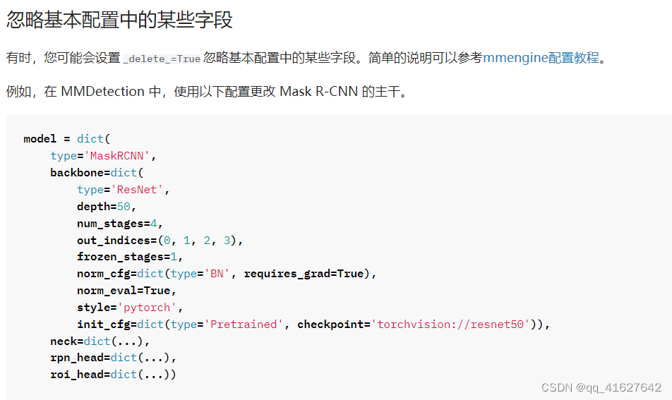

_base_ = '../mask_rcnn/mask-rcnn_r50_fpn_1x_coco.py'
model = dict(
    backbone=dict(
        _delete_=True,
        type='HRNet',
        extra=dict(
            stage1=dict(
                num_modules=1,
                num_branches=1,
                block='BOTTLENECK',
                num_blocks=(4, ),
                num_channels=(64, )),
            stage2=dict(
                num_modules=1,
                num_branches=2,
                block='BASIC',
                num_blocks=(4, 4),
                num_channels=(32, 64)),
            stage3=dict(
                num_modules=4,
                num_branches=3,
                block='BASIC',
                num_blocks=(4, 4, 4),
                num_channels=(32, 64, 128)),
            stage4=dict(
                num_modules=3,
                num_branches=4,
                block='BASIC',
                num_blocks=(4, 4, 4, 4),
                num_channels=(32, 64, 128, 256))),
        init_cfg=dict(type='Pretrained', checkpoint='open-mmlab://msra/hrnetv2_w32')),
    neck=dict(...))
The delete=True would replace all old keys in backbone field with new keys.
(八)使用单级检测器作为 RPN
Use FCOSHead as an RPNHead in Faster R-CNN
Evaluate proposals
Train the customized Faster R-CNN with pre-trained FCOS
1、Use FCOSHead as an RPNHead in Faster R-CNN
要在 Faster R-CNN 中设置FCOSHead,RPNHead我们应该创建一个名为 的新配置文件configs/faster_rcnn/faster-rcnn_r50_fpn_fcos-rpn_1x_coco.py,并将 的设置替换为inrpn_head的设置。此外,我们仍然使用FCOS的颈部设置,步长为,更新为。为了避免损失变为 NAN,我们在前 1000 次迭代而不是前 500 次迭代中应用预热,这意味着 lr 增加得更慢。配置如下:bbox_headconfigs/fcos/fcos_r50-caffe_fpn_gn-head_1x_coco.py[8, 16, 32, 64, 128]featmap_stridesbbox_roi_extractor[8, 16, 32, 64, 128]
_base_ = [
    '../_base_/models/faster-rcnn_r50_fpn.py',
    '../_base_/datasets/coco_detection.py',
    '../_base_/schedules/schedule_1x.py', '../_base_/default_runtime.py'
]

model = dict(
    # copied from configs/fcos/fcos_r50-caffe_fpn_gn-head_1x_coco.py
    neck=dict(
        start_level=1,
        add_extra_convs='on_output',  # use P5
        relu_before_extra_convs=True),
    rpn_head=dict(
        _delete_=True,  # ignore the unused old settings
        type='FCOSHead',
        num_classes=1,  # num_classes = 1 for rpn, if num_classes > 1, it will be set to 1 in TwoStageDetector automatically
        in_channels=256,
        stacked_convs=4,
        feat_channels=256,
        strides=[8, 16, 32, 64, 128],
        loss_cls=dict(
            type='FocalLoss',
            use_sigmoid=True,
            gamma=2.0,
            alpha=0.25,
            loss_weight=1.0),
        loss_bbox=dict(type='IoULoss', loss_weight=1.0),
        loss_centerness=dict(
            type='CrossEntropyLoss', use_sigmoid=True, loss_weight=1.0)),
    roi_head=dict(  # update featmap_strides due to the strides in neck
        bbox_roi_extractor=dict(featmap_strides=[8, 16, 32, 64, 128])))

# learning rate
param_scheduler = [
    dict(
        type='LinearLR', start_factor=0.001, by_epoch=False, begin=0,
        end=1000),  # Slowly increase lr, otherwise loss becomes NAN
    dict(
        type='MultiStepLR',
        begin=0,
        end=12,
        by_epoch=True,
        milestones=[8, 11],
        gamma=0.1)
]
然后,我们可以使用以下命令来训练我们的定制模型
# training with 8 GPUS
bash tools/dist_train.sh configs/faster_rcnn/faster-rcnn_r50_fpn_fcos-rpn_1x_coco.py \
    8 \
    --work-dir ./work_dirs/faster-rcnn_r50_fpn_fcos-rpn_1x_coco
2、Evaluate proposals
The quality of proposals is of great importance to the performance of detector, therefore, we also provide a way to evaluate proposals. Same as above, create a new config file named configs/rpn/fcos-rpn_r50_fpn_1x_coco.py, and replace with setting of rpn_head with the setting of bbox_head in configs/fcos/fcos_r50-caffe_fpn_gn-head_1x_coco.py.
候选区域的质量对于检测器的性能非常重要,因此,我们还提供了一种评估候选框的方法。与上面相同,创建一个名为configs/rpn/fcos-rpn_r50_fpn_1x_coco.py新的配置文件,并将将rpn_head的设置替换为bbox_head的设置在configs/fcos/fcos_r50-caffe_fpn_gn-head_1x_coco.py
_base_ = [
    '../_base_/models/rpn_r50_fpn.py', '../_base_/datasets/coco_detection.py',
    '../_base_/schedules/schedule_1x.py', '../_base_/default_runtime.py'
]

val_evaluator = dict(metric='proposal_fast')
test_evaluator = val_evaluator

model = dict(
    # copied from configs/fcos/fcos_r50-caffe_fpn_gn-head_1x_coco.py
    neck=dict(
        start_level=1,
        add_extra_convs='on_output',  # use P5
        relu_before_extra_convs=True),
    rpn_head=dict(
        _delete_=True,  # ignore the unused old settings
        type='FCOSHead',
        num_classes=1,  # num_classes = 1 for rpn, if num_classes > 1, it will be set to 1 in RPN automatically
        in_channels=256,
        stacked_convs=4,
        feat_channels=256,
        strides=[8, 16, 32, 64, 128],
        loss_cls=dict(
            type='FocalLoss',
            use_sigmoid=True,
            gamma=2.0,
            alpha=0.25,
            loss_weight=1.0),
        loss_bbox=dict(type='IoULoss', loss_weight=1.0),
        loss_centerness=dict(
            type='CrossEntropyLoss', use_sigmoid=True, loss_weight=1.0)))
假设我们在训练后有了检查点./work_dirs/faster-rcnn_r50_fpn_fcos-rpn_1x_coco/epoch_12.pth,那么我们可以使用以下命令评估提案的质量。
# testing with 8 GPUs
bash tools/dist_test.sh \
    configs/rpn/fcos-rpn_r50_fpn_1x_coco.py \
    ./work_dirs/faster-rcnn_r50_fpn_fcos-rpn_1x_coco/epoch_12.pth \
    8
3、使用预训练的 FCOS 训练定制的 Faster R-CNN
预训练不仅可以加快训练的收敛速度,还可以提高检测器的性能。因此,这里我们通过一个例子来说明如何使用预训练的FCOS作为RPN来加速训练并提高准确性。假设我们想使用FCOSHead作 rpn head 在 Faster R-CNN ,在预训练fcos_r50-caffe_fpn_gn-head_1x_coco进行训练。。请注意,fcos_r50-caffe_fpn_gn-head_1x_coco使用 ResNet50 的 caffe 版本,data_preprocessor因此需要更新像素平均值和标准差。
_base_ = [
    '../_base_/models/faster-rcnn_r50_fpn.py',
    '../_base_/datasets/coco_detection.py',
    '../_base_/schedules/schedule_1x.py', '../_base_/default_runtime.py'
]

model = dict(
    data_preprocessor=dict(
        mean=[103.530, 116.280, 123.675],
        std=[1.0, 1.0, 1.0],
        bgr_to_rgb=False),
    backbone=dict(
        norm_cfg=dict(type='BN', requires_grad=False),
        style='caffe',
        init_cfg=None),  # the checkpoint in ``load_from`` contains the weights of backbone
    neck=dict(
        start_level=1,
        add_extra_convs='on_output',  # use P5
        relu_before_extra_convs=True),
    rpn_head=dict(
        _delete_=True,  # ignore the unused old settings
        type='FCOSHead',
        num_classes=1,  # num_classes = 1 for rpn, if num_classes > 1, it will be set to 1 in TwoStageDetector automatically
        in_channels=256,
        stacked_convs=4,
        feat_channels=256,
        strides=[8, 16, 32, 64, 128],
        loss_cls=dict(
            type='FocalLoss',
            use_sigmoid=True,
            gamma=2.0,
            alpha=0.25,
            loss_weight=1.0),
        loss_bbox=dict(type='IoULoss', loss_weight=1.0),
        loss_centerness=dict(
            type='CrossEntropyLoss', use_sigmoid=True, loss_weight=1.0)),
    roi_head=dict(  # update featmap_strides due to the strides in neck
        bbox_roi_extractor=dict(featmap_strides=[8, 16, 32, 64, 128])))

load_from = 'https://download.openmmlab.com/mmdetection/v2.0/fcos/fcos_r50_caffe_fpn_gn-head_1x_coco/fcos_r50_caffe_fpn_gn-head_1x_coco-821213aa.pth'
bash tools/dist_train.sh \
    configs/faster_rcnn/faster-rcnn_r50-caffe_fpn_fcos-rpn_1x_coco.py \
    8 \
    --work-dir ./work_dirs/faster-rcnn_r50-caffe_fpn_fcos-rpn_1x_coco
(九)OHEM 在线难例挖掘
OHEM(Online Hard negative Example Mining,在线难例挖掘)见于[5]。两阶段检测模型中,提出的RoI Proposal在输入R-CNN子网络前,我们有机会对正负样本(背景类和前景类)的比例进行调整。通常,背景类的RoI Proposal个数要远远多于前景类,Fast R-CNN的处理方式是随机对两种样本进行上采样和下采样,以使每一batch的正负样本比例保持在1:3,这一做法缓解了类别比例不均衡的问题,是两阶段方法相比单阶段方法具有优势的地方,也被后来的大多数工作沿用。
论文中把OHEM应用在Fast R-CNN,是因为Fast R-CNN相当于目标检测各大框架的母体,很多框架都是它的变形,所以作者在Fast R-CNN上应用很有说明性。
上图是Fast R-CNN框架,简单的说,Fast R-CNN框架是将224×224的图片当作输入,经过conv,pooling等操作输出feature map,通过selective search 创建2000个region proposal,将其一起输入ROI pooling层,接上全连接层与两个损失层。
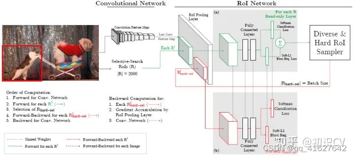
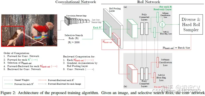
作者将OHEM应用在Fast R-CNN的网络结构,如上图,这里包含两个RoI network,上面一个RoI network是只读的,为所有的RoI 在前向传递的时候分配空间,下面一个RoI network则同时为前向和后向分配空间。在OHEM的工作中,作者提出用R-CNN子网络对RoI Proposal预测的分数来决定每个batch选用的样本。这样,输入R-CNN子网络的RoI Proposal总为其表现不好的样本,提高了监督学习的效率。
首先,RoI 经过RoI plooling层生成feature map,然后进入只读的RoI network得到所有RoI 的loss;然后是hard RoI sampler结构根据损失排序选出hard example,并把这些hard example作为下面那个RoI network的输入。
实际训练的时候,每个mini-batch包含N个图像,共|R|个RoI ,也就是每张图像包含|R|/N个RoI 。经过hard RoI sampler筛选后得到B个hard example。作者在文中采用N=2,|R|=4000,B=128。 另外关于正负样本的选择:当一个RoI 和一个ground truth的IoU大于0.5,则为正样本;当一个RoI 和所有ground truth的IoU的最大值小于0.5时为负样本。
总结来说,对于给定图像,经过selective search RoIs,同样计算出卷积特征图。但是在绿色部分的(a)中,一个只读的RoI网络对特征图和所有RoI进行前向传播,然后Hard RoI module利用这些RoI的loss选择B个样本。在红色部分(b)中,这些选择出的样本(hard examples)进入RoI网络,进一步进行前向和后向传播。
MMDetection中,OHEM(online hard example mining):(源码解析)
rcnn=[
        dict(
            assigner=dict(
                type='MaxIoUAssigner',
                pos_iou_thr=0.4, # 更换
                neg_iou_thr=0.4,
                min_pos_iou=0.4,
                ignore_iof_thr=-1),
            sampler=dict(
                type='OHEMSampler',
                num=512,
                pos_fraction=0.25,
                neg_pos_ub=-1,
                add_gt_as_proposals=True),
            pos_weight=-1,
            debug=False),
        dict(
            assigner=dict(
                type='MaxIoUAssigner',
                pos_iou_thr=0.5,
                neg_iou_thr=0.5,
                min_pos_iou=0.5,
                ignore_iof_thr=-1),
            sampler=dict(
                type='OHEMSampler', # 解决难易样本,也解决了正负样本比例问题。
                num=512,
                pos_fraction=0.25,
                neg_pos_ub=-1,
                add_gt_as_proposals=True),
            pos_weight=-1,
            debug=False),
        dict(
            assigner=dict(
                type='MaxIoUAssigner',
                pos_iou_thr=0.6,
                neg_iou_thr=0.6,
                min_pos_iou=0.6,
                ignore_iof_thr=-1),
            sampler=dict(
                type='OHEMSampler',
                num=512,
                pos_fraction=0.25,
                neg_pos_ub=-1,
                add_gt_as_proposals=True),
            pos_weight=-1,
            debug=False)
    ],
    stage_loss_weights=[1, 0.5, 0.25])
MMSegmention中,OHEM(online hard example mining):(源码解析
我们实现了像素采样器来进行训练采样,例如 OHEM(在线困难示例挖掘),它用于删除模型训练中的“简单”示例。以下是启用 OHEM 的训练 PSPNet 的示例配置。
_base_ = './pspnet_r50-d8_4xb2-40k_cityscapes-512x1024.py'
model=dict(
    decode_head=dict(
        sampler=dict(type='OHEMPixelSampler', thresh=0.7, min_kept=100000)) )
这样,只有置信度得分低于0.7的像素才被用来训练。并且我们在训练期间至少保留 100000 个像素。如果thresh未指定,min_kept则将选择顶部损失的像素。
(十) 类别平衡损失
对于类别分布不平衡的数据集,您可以更改每个类别的损失权重。这是城市景观数据集的示例。
_base_ = './pspnet_r50-d8_4xb2-40k_cityscapes-512x1024.py'
model=dict(
    decode_head=dict(
        loss_decode=dict(
            type='CrossEntropyLoss', use_sigmoid=False, loss_weight=1.0,
            # DeepLab used this class weight for cityscapes
            class_weight=[0.8373, 0.9180, 0.8660, 1.0345, 1.0166, 0.9969, 0.9754,
                        1.0489, 0.8786, 1.0023, 0.9539, 0.9843, 1.1116, 0.9037,
                        1.0865, 1.0955, 1.0865, 1.1529, 1.0507])))
(十一)Soft NMS 软化非极大抑制
(十二)RoIAlign RoI对齐
(十三)GIoULoss
(十四)是时候该学会 MMDetection 进阶之非典型操作技能(一)
(十五)ResNet 高精度预训练模型在 MMDetection 中的最佳实践
(十六) Box Refinement/Voting 预测框微调/投票法/模型融合
(十七)mmdetection中如何实现SWA(Stochastic Weight Averaging)
mmdetection中如何实现SWA(Stochastic Weight Averaging)
swa 物体检测 第4414章
我们在目标检测器训练过程中添加了SWA 训练阶段


 309
309


 被折叠的 条评论
为什么被折叠?
被折叠的 条评论
为什么被折叠?
 到【灌水乐园】发言


