【RNN详解】SimpleRNN，LSTM，bi-LSTM的原理及Tensorflow实现

最新推荐文章于 2025-04-17 22:02:23 发布

Sciengineer-Mike

最新推荐文章于 2025-04-17 22:02:23 发布

阅读量2.6k

点赞数 1

文章标签： tensorflow rnn lstm

本文链接：https://blog.csdn.net/qq_43018832/article/details/128423975

版权

1.摘要

RNN是一种特殊的神经网络结构，它是根据“人的认知是基于过往的经验和记忆”这一观点提出的，它与DNN，CNN不同的是：它不仅考虑前一时刻的输入，而且赋予了网络对前面内容的一种“记忆”功能，对于处理序列数据比较友好。RNN之所以称为循环神经网路，即一个序列当前的输出与前面的输出也有关。具体的表现形式为网络会对前面的信息进行记忆并应用于当前输出的计算中，即隐藏层之间的节点不再无连接而是有连接的，并且隐藏层的输入不仅包括输入层的输出还包括上一时刻隐藏层的输出。本篇将分别介绍SimpleRNN，LSTM，bi-LSTM。

2.SimpleRNN

2.1.原理介绍

在介绍之前，我们先来认识下最简单的SimpleRNN，如下图，我们先看左边X-U-S-V-O这条路线，这就好比一个全连接神经网络，X为输入数据，U为输入层到隐藏层的权重矩阵，S为隐藏层，V为隐藏层到输出层O的权重矩阵。如果加上W，隐藏层S的值不仅仅取决于输入层X，还取决于上次隐藏层的值与权重矩阵W相乘的值，相信大家都可以理解。按时间先展开，如右侧所示。
在这里插入图片描述
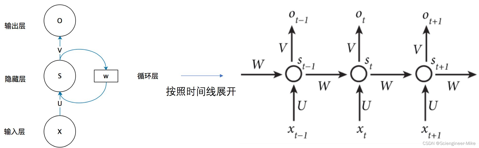
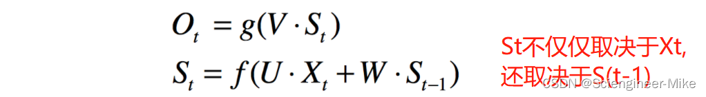
我们可以用如下公式来表示上图的关系：

2.2.代码实现

接下来，我们使用keras中的SimpleRNN模型对IMDB数据集进行训练，代码如下：

from tensorflow.keras.datasets import imdb
from tensorflow.keras.preprocessing import sequence
# 作为特征的单词个数
max_features = 10000 
# 在maxlen个单词后截断文本
maxlen = 500 
batch_size = 32
print('Loading data...')
(input_train, y_train), (input_test, y_test) = imdb.load_data(num_words=max_features)
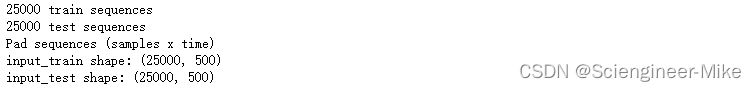
print(len(input_train), 'train sequences')
print(len(input_test), 'test sequences')
print('Pad sequences (samples x time)')
input_train = sequence.pad_sequences(input_train, maxlen=maxlen)
input_test = sequence.pad_sequences(input_test, maxlen=maxlen)
print('input_train shape:', input_train.shape)
print('input_test shape:', input_test.shape)

在这里插入图片描述

from tensorflow.keras.layers import Dense,Embedding,SimpleRNN
from tensorflow.keras.models import Sequential
# 搭建模型
model = Sequential() 
model.add(Embedding(max_features, 32)) 
model.add(SimpleRNN(32)) 
model.add(Dense(1, activation='sigmoid'))
model.compile(optimizer='rmsprop', loss='binary_crossentropy', metrics=['acc'])
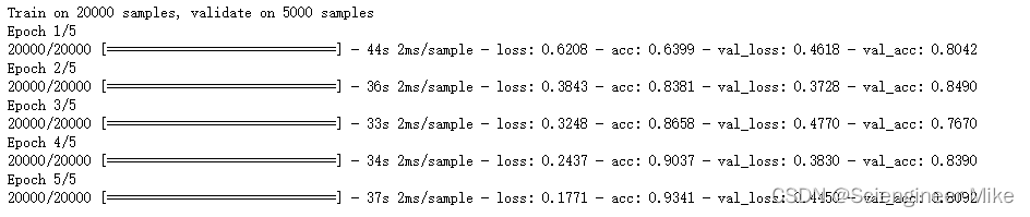
history = model.fit(input_train, y_train,
                    epochs=5, 
                    batch_size=128,
                    validation_split=0.2)

在这里插入图片描述

3.LSTM

3.1.原理介绍

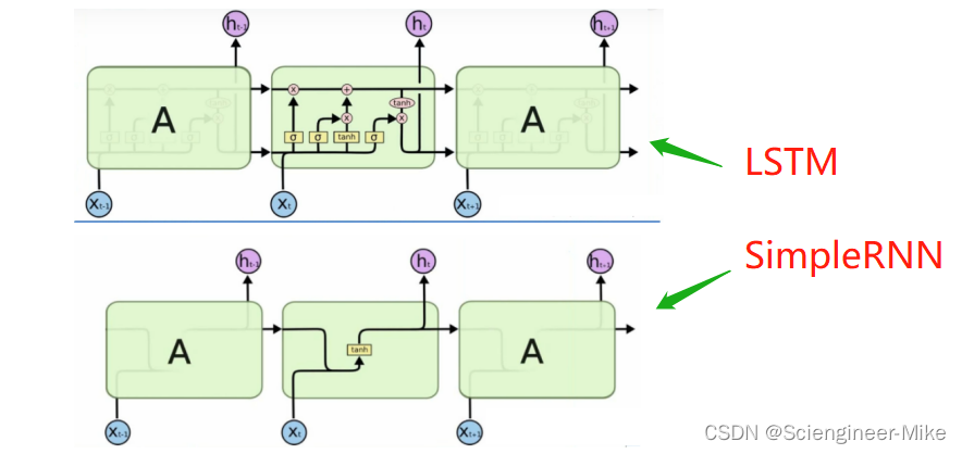
接下来，来讲RNN里面的算法之星LSTM，是一种改进后的循环神经网络，可以解决simpleRNN无法处理长距离的依赖问题以及梯度爆炸的问题，目前比较流行。相比于原始的RNN的隐层(hidden state)， LSTM增加了一个记忆细胞（如下图），具有选择性记忆功能，可以选择记忆重要信息，过滤掉噪音信息，减轻记忆负担。
在这里插入图片描述
LSTM模型解读：
（1）遗忘门

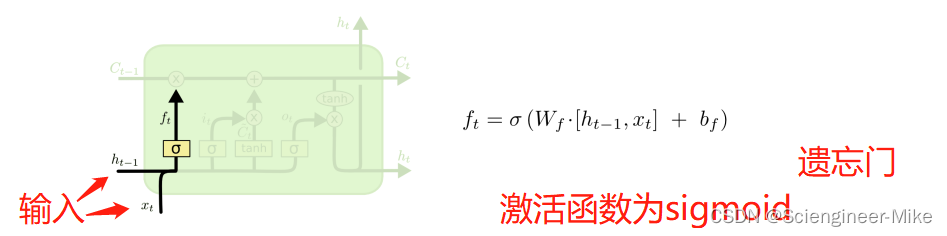
遗忘门的输入为Xt和h(t-1)，输出是ft，激活函数为sigmoid函数，激活函数使ft的输出范围为0-1之间，当值为0时，后续与C(t-1)相乘时，结果为0，即“遗忘”，因此叫做遗忘门，结果还是十分简单的。
（2）更新门
在这里插入图片描述
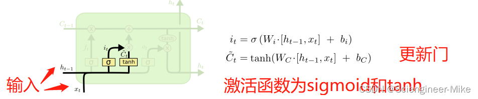
更新门输入也是h(t-1)和Xt，输出分别为it（和遗忘门一样）和C`t（更新的信息），对应的激活函数为sigmoid和tanh，sigmoid输出结果为（0，1），tanh输出结果为（-1，1）。

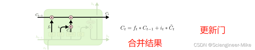
如上图所示，C(t-1)和ft相乘，it和C’t相乘，前者代表对过去信息选择性的保留，后者代表更新的信息的添加，最后将两部分合并起来，就是新的状态Ct了。
（3）输出门层
在这里插入图片描述
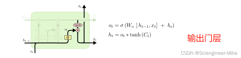
这就是LSTM模型的输出了，Ot是h(t-1)和Xt输入后经sigmoid后的结果，Ct通过tanh缩放后与Ot相乘，就是输出了。

3.2.代码实现

说了半天原理，接下来使用keras中的LSTM模型对IMDB数据集进行训练，代码如下：

from tensorflow.keras.datasets import imdb
from tensorflow.keras.preprocessing import sequence
# 作为特征的单词个数
max_features = 10000 
# 在maxlen个单词后截断文本
maxlen = 500 
batch_size = 32
print('Loading data...')
(input_train, y_train), (input_test, y_test) = imdb.load_data(num_words=max_features)
print(len(input_train), 'train sequences')
print(len(input_test), 'test sequences')
print('Pad sequences (samples x time)')
input_train = sequence.pad_sequences(input_train, maxlen=maxlen)
input_test = sequence.pad_sequences(input_test, maxlen=maxlen)
print('input_train shape:', input_train.shape)
print('input_test shape:', input_test.shape)

在这里插入图片描述

from tensorflow.keras.models import Sequential
from tensorflow.keras.layers import Dense, Dropout, Activation,Flatten
from tensorflow.keras.layers import Embedding
from tensorflow.keras.layers import LSTM
# 搭建模型
model = Sequential()
model.add(Embedding(max_features, 32))
# 加LSTM
model.add(LSTM(32))
model.add(Dense(units=256,activation='relu' ))
model.add(Dropout(0.2))
model.add(Dense(units=1,activation='sigmoid' ))
model.compile(loss='binary_crossentropy', optimizer='adam',metrics=['accuracy'])

train_history =model.fit(input_train, y_train,batch_size=128, 
                         epochs=5,validation_split=0.2)

在这里插入图片描述
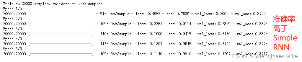
由以上结果，可以看出LSTM的准确率高于SimpleRNN。

4.LSTM改进—bi_LSTM

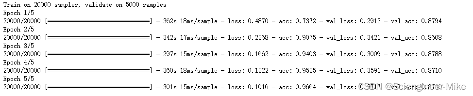
在单向的循环神经网络中，模型实际上只使用到了“上文”的信息，而没有考虑到“下文”的信息。在实际场景中，预测可能需要使用到整个输入序列的信息。因此，目前业内主流使用的都是双向的循环神经网络。顾名思义，双向循环神经网络结合了序列起点移动的一个循环神经网络和令一个从序列末尾向序列起点移动的循环神经网络。而作为循环神经网络的一种拓展，LSTM 自然也可以结合一个逆向的序列，组成双向长短时记忆网络(Bi-directional Long Short-Term Memory, Bi-LSTM)。Bi-LSTM 目前在自然语言处理领域的应用场景很多，并且都取得了不错的效果。具体原理不在多述，直接上代码看效果。
代码实现：

from tensorflow.keras.datasets import imdb
from tensorflow.keras.preprocessing import sequence
# 作为特征的单词个数
max_features = 10000 
# 在maxlen个单词后截断文本
maxlen = 500 
batch_size = 32
print('Loading data...')
(input_train, y_train), (input_test, y_test) = imdb.load_data(num_words=max_features)
print(len(input_train), 'train sequences')
print(len(input_test), 'test sequences')
print('Pad sequences (samples x time)')
input_train = sequence.pad_sequences(input_train, maxlen=maxlen)
input_test = sequence.pad_sequences(input_test, maxlen=maxlen)
print('input_train shape:', input_train.shape)
print('input_test shape:', input_test.shape)

在这里插入图片描述

from tensorflow.keras.models import Sequential
from tensorflow.keras.layers import Dense, Dropout, Activation,Flatten
from tensorflow.keras.layers import Embedding
from tensorflow.keras.layers import Bidirectional,LSTM

model = Sequential()
model.add(Embedding(max_features, 32))
model.add(Bidirectional(LSTM(32)))
model.add(Dense(units=256,activation='relu' ))
model.add(Dropout(0.2))
model.add(Dense(1, activation='sigmoid'))

# 尝试使用不同的优化器和不同的优化器配置
model.compile('adam', 'binary_crossentropy', metrics=['accuracy']) 
model.fit(input_train, y_train,batch_size=128,
          epochs=5,validation_split=0.2)

在这里插入图片描述

5.总结

本篇主要讲解了RNN循环神经网络，首先讲了最简单的SimpleRNN，讲解了其实现原理，并用其实现了IMDB影评情感分析，接下来，通过SimpleRNN引出了LSTM，分析了二者之间的区别，以及LSTM网络结构上的创新，最后介绍了可以双向传播的bi-LSTM，具有更好的记忆功能，其在实际应用中使用广泛。希望对读者的学习有一定的帮助。