基于集合的粒子群算法（S-PSO）求解车辆路径优化问题

VRP问题空间（problem space）可以看成完全图$G=(V,A)$，问题的解则为$G$的生成子图。

• 简单图（simple graph）：若一个图中没有自环和重边，则是简单图。具有至少两个顶点的简单无向图中一定存在度相同的结点（鸽巢原理）。
• 完全图（complete graph）： 也称简单完全图。假设一个图有n个顶点，那么如果任意两个顶点之间都有边的话，该图就称为完全图。
• 哈密顿回路（Hamilton circle）： G=(V,E)是一个图，若G中一条路径通过且仅通过每一个顶点一次，称这条路径为哈密顿路径。若G中一个回路通过且仅通过每一个顶点一次，称这个环为哈密顿回路。若一个图存在哈密顿回路，就称为哈密顿图。
  • 简而言之，哈密尔顿回路是指，从图中的一个顶点出发，沿着边行走，经过图的每个顶点，且每个顶点仅访问一次，之后再回到起始点的一条路径。

一、粒子群算法（Traditional Particle Swarm Optimization，PSO）

粒子群算法用于解决连续问题，粒子按速度更新公式（1）和位置更新公式（2）寻找最优解：
$$\begin{array}{rl}{v}_i^j& \leftarrow \omega v_i^j+c_1{r}_1(pbes{t}_i^j-x_i^j)+c_2{r}_2(gbes{t}^j-x_i^j)\\ x_i^j& \leftarrow x_i^j+v_i^j\end{array}$$
其中，

• $D$——代表搜索空间为D维（即为自变量的个数）。$j$粒子维度索引，$j=1,2,...,D$。
• $x_i$——代表第$i$个粒子的位置（即为一个解)，$x_i=(x_i^1,x_i^2,...,x_i^j,...,x_i^D)$。
• $v_i$——代表第$i$个粒子的速度，$v_i=(v_i^1,v_i^2,...,v_i^j,...,v_i^D)$。
• $pbes{t}_i$——代表粒子$i$在搜索到的最优位置，$pbes{t}_i=(pbes{t}_i^1,pbes{t}_i^2,...,pbes{t}_i^j,...,pbes{t}_i^D)$。
• $gbes{t}^j$——整个鸟群搜索到的最优位置。$gbes{t}^j$和 $pbes{t}_i^j$关系为： g b e s t j = min ⁡ { p b e s t i j } j = 1 D gbest^{j}= \min \{pbest_{i}^j\}_{j=1}^D gbestj=min{pbestij​}j=1D​
• $\omega$——惯性权重(inertia weight)，动态调整惯性权重可以平衡收敛的全局性和收敛速度。$\omega$越大，探索新区域的能力越强，有利于全局搜索，跳出局部最优；$\omega$越小，逐渐退化成爬山算法，有利于算法收敛。推荐取值范围$\omega \in [0.4,2]$，另有实验表明$\omega =0.7298$时，算法有较好的收敛性能。
• $c_1$——加速系数，表征粒子个体的经验，该值越大，证明鸟群在寻找食物过程中，越倾向于根据自己的经验知识寻找食物；该值越小，表示不注重自己的经验，鸟在寻找食物过程中“随大流、从众”。
• $c_2$——加速系数，表征整个鸟群的经验知识，该值越大，越注重鸟之间的信息共享；该值越小，鸟之间没有信息交流，算法演变为随机探索，导致算法收敛速度缓慢。
  实验表明，$c_1=c_2=1.479$时算法有较好的收敛性能。

二、离散粒子群算法（Discrete PSO）

为了将PSO的思想应用于求解离散优化问题，研究人员在文献中提出了几种PSO离散化的方法。

离散二进制PSO（Binary PSO，BPSO）

基本PSO是用来解决连续问题优化的，离散二进制PSO用来解决组合优化问题。在离散空间中扩展粒子群算法最简单的方法是二进制粒子群算法(BPSO)。在BPSO中，每个决策变量xi只能为0或1，而其对应的速度vi表示为1的概率。粒子群算法的发起者Kennedy和Eberhart[15]首先在粒子群算法中引入二进制编码，利用sigmoid变换函数控制位置更新的输出。随后，又提出了角度调制和多相等BPSO速度和位置更新策略[14,17]。最近，Liu等人[16]引入了一个理论模型来分析BPSO的搜索行为，并进一步发展了一种自适应惯性权重方案。

总体而言，BPSO在背包问题、网络聚类问题和组播路由问题等离散优化问题上取得了令人满意的性能。然而，BPSO只能支持二进制编码。对于许多基于排列的组合优化问题（permutation-based COPs），要找到一个合理和直观的二进制表示方案并不容易。因此，有必要探索一种更灵活的方法来扩展粒子群算法在离散空间中的应用。

基于交换算子的PSO（基于交换算子的PSO）

另一种应用于离散优化问题的方法是基于交换算子的粒子群优化算法。在这种方法中，粒子的位置和速度分别定义为一组数字的排列和一组交换。首先，Clerc[21]设计了第一个版本的基于交换算子的PSO，用于解决经典的旅行推销员问题(TSP)。根据[21]，粒子的位置被重新定义为一个城市的排列，粒子的速度被重新定义为一个交换算子的集合，这些交换算子在城市的排列中交换多个城市的位置。类似地，Wang et al.[22]提出了另一种基于交换算子的离散PSO算法来解决TSP问题，Rameshkumar et al.[24]提出了一种基于交换算子的PSO算法来处理置换流水车间调度问题(permutation flow-shop scheduling problem, FSP)。最近，Huang et al.[23]开发了一种改进的基于交换算子的PSO，该PSO通过种子和扩展策略来解决网络对齐问题(NAP)。

然而，由于基于交换算子的速度的特殊定义，使得基于交换算子的粒子群优化算法在基于置换优化问题中的应用受到限制。

Space transformation approach

空间变换是扩展粒子群算法求解COPs的另一种方法[25-29]。与其他离散PSO算法不同的是，该算法将粒子在实空间中演化，然后利用空间变换技术将连续向量转换为离散解向量。例如Salman等人[26]提出了一种基于轮函数的离散PSO算法来解决任务分配问题。为了解决多目标网格调度问题，Zhu和Wang[28]提出了一种离散PSO算法，该算法采用了一种基于深度阶和相对阶的空间变换技术。

虽然这类算法仍然可以使用原粒子群算法的位置和速度更新规则，但对于离散搜索空间来说，连续表示是冗余的。换句话说，问题的一个解决方案可以映射到连续搜索空间中的多个位置，这可能会降低搜索性能。此外，针对不同问题的空间转换设计大多是临时性的。对于复杂的cop，设计一种有效的空间变换方法通常并不容易。

混合离散粒子群算法（Hybrid discrete PSO）

也有许多方法将粒子群算法与其他技术相结合来求解离散优化问题[30 - 41]。综上所述，这些混合算法可分为三类:1)将PSO与其他计算智能算法相结合[32,33,39 - 41];2)将PSO与辅助的问题相关搜索策略相结合[30,31,36];3)将PSO与局部搜索方法相结合[34,35,37]。
总体而言，将粒子群算法与其他优化方法相结合，可以有效地解决TSP[37]、VRP[36]、JSP[33]等各种离散优化问题。然而，现有的混合方法主要是针对具体问题设计的。因此，它们通常不适用于其他问题。此外，混合粒子群算法通常比其他离散粒子群算法更加复杂和难以实现。

三、基于集合的粒子群算法（set-based Particle Swarm Optimizatio，S-PSO）

为了缓解现有离散PSO算法的不足，为在离散空间中使用PSO算法开发一个更通用和灵活的框架，在[42]中提出了一套为基础的PSO (S-PSO)框架。离散变量天然可以用集合进行表示，S-PSO在集合空间中重新定义了PSO。（Based on the fact that a set is a natural representation for discrete variables, S-PSO redefines the concepts of PSO in the set space。）

基于S-PSO的旅行商问题（Travelling Salesman Problem, TSP）建模求解

VRP问题是permutation-based problem，问题空间（problem space）可以看成完全图$G=(V,A)$，问题的解则为$G$的生成子图（spanning subgraph），以旅行商问题为例，速度和位置按如下方式定义。

初始解构造方式：

• 随机选择一个节点（城市）作为出发点。
• 选择与上一步中选择的节点相邻的可行弧加入到路径中。
• 移动到当前路径的终点，重复步骤2)，直到建立一个完整的哈密顿回路\

3.1 重新定义位置和速度

对经典连续粒子群算法重的位置和速度进行重新定义：

• 全集$E$是TSP问题中边$(i,j)$的集合，$E^j$是和点$j$相关的边的集合

位置（Position）

一个粒子的位置就是问题的一个可行解。第$i$个粒子的位置用$X_i$（$X_i\subseteq E$）表示，$X_i=[X_i^0,X_i^1,...,X_i^j,...,X_i^n]$。算法初始化$X_i$为随机生成的可行解，如$X_i$即为$[(1,2),(2,3),(3,4),(4,1)]$。

速度（Velocity）

在S-PSO中，定义速度为一个带概率的集合，第$i$个粒子的速度表示为 V i = { e / p ( e ) ∣ e ∈ E } V_i= \{e/p(e)|e \in E\} Vi​={e/p(e)∣e∈E}。$V_i$中的概率$p(e)$实际上提供了粒子$i$将从元素$e$学习构造新位置的可能性。

其中：$E$是全集；$p(e)\in [0,1]$

3.2 重新定义操作运算符

系数$\times$速度

c V = { e / p ′ ( e ) } cV=\{e/p^\prime(e)\} cV={e/p′(e)}

$p^{\prime }(e)=\{\begin{array}{ll}1& \text{if}c\times p(e)>1\\ c\times p(e)& \text{otherwise}\end{array}$

V i j = { e / p ( e ) ∣ e ∈ E j } V_i^j = \{e/p(e)|e \in E^j\} Vij​={e/p(e)∣e∈Ej}。

位置-位置

给定两个集合$A$和$B$， A − B = { e ∣ e ∈ A and e ∉ B } A-B=\{e| e\in A\quad\text{and} \quad e \notin B\} A−B={e∣e∈Aande∈/B}。基于这个定义则可以计算$Gbes{t}^j-X_i^j$和$Pbes{t}_i^j-X_i^j$，即找出$Gbest(Pbes{t}_i)$中有的元素而$X_i$中没有的元素，这些元素有潜在的可能性改善解$X_i$的质量。

系数$\times$位置
给定系数c和集合$E^{\prime }$：
c E ′ = { e / p ′ ( e ) ∣ e ∈ E } cE^\prime=\{e/p^\prime(e)|e\in E\} cE′={e/p′(e)∣e∈E}，$p^{\prime }(e)=\{\begin{array}{ll}1& \text{if}c\times p(e)>1\\ c& \text{otherwise}\\ 0& \text{if}e\notin E^{\prime }\end{array}$

速度+速度

给定两个速度 V 1 = { e / p 1 ( e ) ∣ e ∈ E } V_1=\{e / p_1 (e) | e ∈ E\} V1​={e/p1​(e)∣e∈E}， V 2 = { e / p 2 ( e ) ∣ e ∈ E } V_2=\{e / p_2 (e) | e ∈ E\} V2​={e/p2​(e)∣e∈E}：
V 1 + V 2 = { e / max ⁡ ( p 1 ( e ) , p 2 ( e ) ) ∣ e ∈ E } V_1+V_2=\{e/ \max(p_1(e), p_2(e))|e \in E\} V1​+V2​={e/max(p1​(e),p2​(e))∣e∈E}

3.3速度更新和位置更新

速度更新

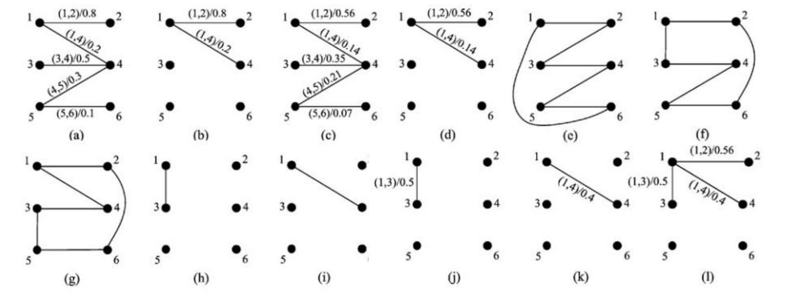
通过重新定义操作运算符，则可以按照式（1）更新速度，例如：

• （a）第$i$个粒子的速度$V_i=\{(1,2)/0.8,(1,4)/0.2,(3,4)/0.5,(4,5)/0.3,(5,6)/0.1\}$。

• （b）$V_i^j$即第$i$个粒子在第$j$个维度的速度，$V_i^1=\{(1,2)/0.8,(1,4)/0.2\}$，

• （c）（d）$\omega V_i^j$即第$j$维的速度乘上系数$\omega$，$\omega V_i^1=\{(1,2)/0.56,(1,4)/0.14\}$，其中$\omega =0.7,j=1$。

• （e）$X_i=\{(1,2),(2,3),(3,4),(4,5),(5,6),(1,6)\}$为第$i$个粒子的位置，是一个可行解，$X_i^1=\{(1,2),(1,6)\}$；

• （f）$GBest$指在整个粒子群历史最优解$X_i=\{(1,2),(2,6),(6,5),(4,5),(4,3),(3,1)\}$，$GBes{t}_i^1=\{(1,2),(3,1)\}$

• （g）$PBes{t}_i$指第 $i$ 个粒子找到过的历史最优解；$PBes{t}_i=\{(1,2),(2,6),(6,5),(3,5),(4,3),(4,1)\}$，$PBes{t}_i^1=\{(1,2),(1,4)\}$

• （h）$GBes{t}^1-X_i^1=\{(1,2),(3,1)\}-\{(1,2),(1,6)\}=\{(3,1)\}$；

• （i）$PBes{t}_i^1-X_i^1=\{(1,2),(1,4)\}-\{(1,2),(1,6)\}=\{(1,4)\}$

• （j）$c_2{r}_2^1(GBes{t}^1-X_i^1)=\{(3,1)/0.5\}$，其中$c_2{r}_2^1=0.5$

• （k）$c_1{r}_1^1=0.4$，则$c_1{r}_1^1(PBes{t}_i^1-X_i^1)=\{(1,4)/0.4\}$

• （l）更新后的$V_i{}^1\leftarrow V_i^1+c_1{r}_1^1(PBes{t}_i^1-X_i^1)+c_2{r}_2^1(GBes{t}^1-X_i^1)=\{(1,2)/0.56,(1,4)/0.4,(3,1)/0.5\}$

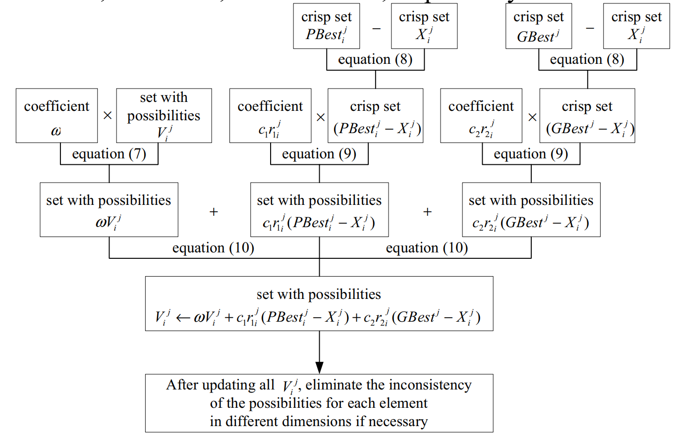
有$PBes{t}_i^j、X_i^j、Ges{t}^j、V_i^j$及惯性因子$\omega$、个体因子$c_1$、社会因子$c_2$，速度更新过程如下图。

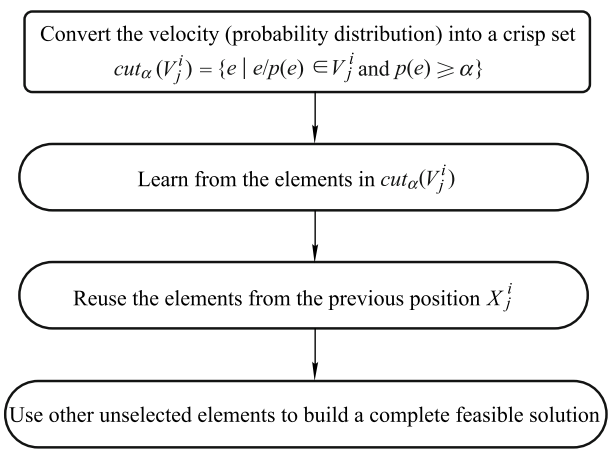
位置更新

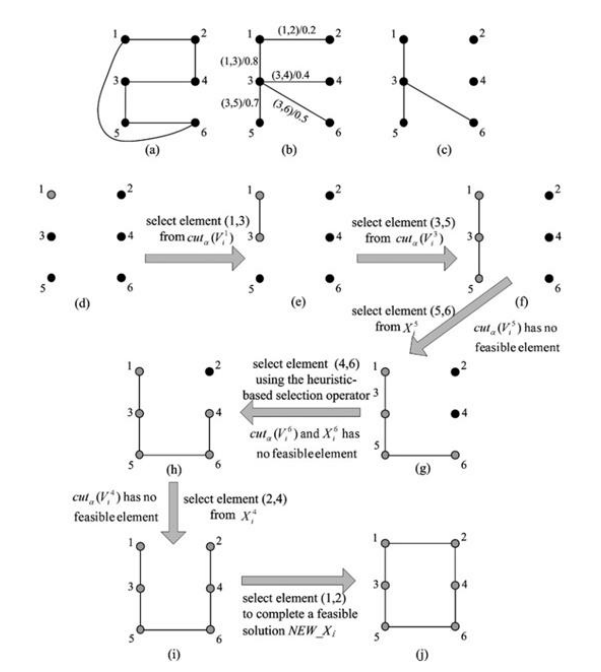
更新速度后，粒子i使用新的速度vit调整其当前位置Xi，并构建一个新的位置NEW_Xi。与连续空间中的情况不同，离散空间中的位置必须满足约束Ω .为了保证NEW_Xi的可行性，在S-PSO中，第i个粒子应用图2中给出的位置更新过程position_updatatin (Xi,Vi)来构建新位置。即在inS-PSO中，粒子i更新其位置的方式如下：

1. 由$V_i^j$生成一个新的集合${\text{Cut}}_{\alpha }(V_i^j)$，其中 Cut α ( V i j ) = { e / p ( e ) ∈ V i j  and  p ( e ) ≥ α } \text{Cut}_{\alpha}(V_{i}^j)=\{e/p(e) \in V_i^j\ \text{and}\ p(e) \geq \alpha\} Cutα​(Vij​)={e/p(e)∈Vij​ and p(e)≥α}，$\alpha \in (0,1)$是一个随机数。
2. 设新解 X i ′ = { } X_i^\prime=\{\} Xi′​={}，对于每一个维度$j$，从${\text{Cut}}_{\alpha }(V_i^j)$选择元素加入到$X_i^{\prime }$。如果${\text{Cut}}_{\alpha }(V_i^j)$不存在$j$维度的元素，则从原解$X_i$中选择元素。如果$X_i$中仍没有，则从全集$E$中选择元素，直至$X_i$构造完成。

举例说明

对于有$n=4$个城市的TSP问题（对称TSP，symmetric TSP）：

初始化全集$E$，粒子的位置和速度：

• 全集$E=\{(1,2),(1,3),(1,4),(2,3),(2,4),(3,4)\}$；

  • $E^1=\{(1,2),(1,3),(1,4)\}$
  • $E^2=\{(1,2),(2,3),(2,4)\}$
  • $E^3=\{(1,3),(2,3),(3,4)\}$
  • $E^4=\{(1,4),(2,4),(3,4)\}$

• 若一个可行解为$[1,2,3,4]$，位置表示为$X=\{(1,2),(2,3),(3,4),(1,4)\}$

  • $X^1=\{(1,2),(1,4)\}$
  • $X^2=\{(1,2),(2,3)\}$
  • $X^3=\{(2,3),(3,4)\}$
  • $X^4=\{(3,4),(1,4)\}$

初始化第i个粒子的速度$V_i$：
随机从全集$E$中选择$n$个元素，并为每个元素生成一个概率$p(e)\in [0,1]$

完整代码（Python）

使用att48进行测试，对于对称TSP，边(i,j)和边(j,i)是等价的，因此重写hashcode和equals方法，并且重新定义速度类和位置类，实现操作运算符的重载。

import collections
import copy
import itertools
import random
import threading
import multiprocessing
import time

import matplotlib.pyplot as plt
import numpy as np

from typing import *
from numpy import ndarray
from scipy import spatial


def timer(func):
    def inner(*args, **kwargs):
        start = time.time()
        gbest = func(*args, **kwargs)
        end = time.time()
        print(f'程序运行时间：{round(end - start, 2)}s')
        return gbest

    return inner


class Arc:
    def __init__(self, from_node, to_node):
        self.arc = (from_node, to_node)
        self.from_node = from_node
        self.to_node = to_node

    def get_to_node(self, from_node):
        start, end = self.arc
        if start == from_node:
            return end
        else:
            return start

    def __hash__(self):
        return hash(self.from_node + self.to_node)

    def __eq__(self, other):
        self_i, self_j = self.arc
        other_i, other_j = other.arc
        return self.arc == other.arc or (self_i == other_j and self_j == other_i)

    def __rmul__(self, coeff):
        if coeff > 1:
            coeff = 1
        return self, coeff

    def __contains__(self, node):
        return self.from_node == node or self.to_node == node

    def __repr__(self):
        return f"{self.arc}"


class MySet(set):
    hashset: Set = None

    def __init__(self, hashset=None):
        super().__init__()
        self.hashset: Set = hashset if hashset is not None else set()

    def __rmul__(self, coeff):
        hashmap = {}
        for arc in self.hashset:
            arc, coeff = coeff * arc
            hashmap[arc] = coeff
        return ProbabilitySet(hashmap)  # MySet[Tuple, Tuple,...]

    def __add__(self, other):
        pass

    def __sub__(self, other):
        return MySet(self.hashset - other.hashset)

    def __repr__(self):
        return f'{self.hashset}'


class ProbabilitySet:
    hashmap: Dict[Arc, float] = None

    def __init__(self, hashmap):
        self.hashmap = hashmap if hashmap is not None else {}

    def __add__(self, other):
        union = self.hashmap.keys() | other.hashmap.keys()
        new_velocity = {}
        for edge in union:
            new_velocity[edge] = max(self.hashmap.get(edge, 0), other.hashmap.get(edge, 0))
        return ProbabilitySet(new_velocity)

    def __rmul__(self, coeff):
        hashmap = {}
        for edge, prob in self.hashmap.items():
            prob = coeff * prob
            if prob > 1:
                hashmap[edge] = 1
            else:
                hashmap[edge] = prob
        return ProbabilitySet(hashmap)

    def __repr__(self):
        return f'{self.hashmap}'


class TSP(object):
    num_city: int = None  # 城市数量
    city_coord: Dict[int, Tuple[int, int]] = None  # 城市标号及对应坐标，示例 1：(23,312)
    distance: ndarray = None  # 城市间距离矩阵

    def __init__(self, city_coord):
        self.num_city = len(city_coord)
        self.city_coord = city_coord
        self.city_list = city_coord.keys()
        self.coord_list = np.asarray(list(city_coord.values()))
        self.distance = spatial.distance.cdist(self.coord_list, self.coord_list, 'euclidean')


class Position:
    def __init__(self, path=None):
        if path is not None:
            path = list(path)
            path.append(path[0])
            self.position = collections.defaultdict(set)
            for i, j in itertools.pairwise(path):
                self.position[i].add(Arc(i, j))
                self.position[j].add(Arc(i, j))
        else:
            self.position = collections.defaultdict(set)

    def put(self, d, e):
        self.position[d] = e

    def pop(self, key):
        self.position.pop(key)

    def __len__(self):
        return len(self.position)

    def __getitem__(self, d):
        return MySet(self.position[d])

    def __repr__(self):
        return f'{self.position}'


class Velocity():
    def __init__(self):
        self.dimension: Dict[Tuple[Arc, float]] = {}
        # self.vel = MySet()
        self.velocity: Dict[Arc, float] = {}

    # def add(self, __element) -> None:
    #     self.vel.add(__element)

    def put(self, edge, prob):
        self.velocity[edge] = prob

    def update(self, hashset: ProbabilitySet) -> None:
        self.velocity.update(hashset.hashmap)

    def update_dimension(self):
        if not self.velocity:
            raise RuntimeError("更新速度为空!")

        self.dimension = collections.defaultdict(set)
        for edge, prob in self.velocity.items():
            edge_prob = (edge, prob)
            self.dimension[edge.from_node].add(edge_prob)
            self.dimension[edge.to_node].add(edge_prob)

    def __len__(self):
        return len(self.velocity)

    def __getitem__(self, d) -> ProbabilitySet:
        hashmap = {}
        for edge, prob in self.dimension[d]:
            hashmap[edge] = prob
        return ProbabilitySet(hashmap)

    def __repr__(self):
        return f'{self.velocity}'


class MyThread(threading.Thread):
    def __init__(self, func, args):
        '''
        :param func: 可调用的对象
        :param args: 可调用对象的参数
        '''
        threading.Thread.__init__(self)
        self.func = func
        self.args = args
        self.result = None

    def run(self):
        self.result = self.func(*self.args)

    def getResult(self):
        return self.result


class MyProcess(multiprocessing.Process):
    def __init__(self, func, args):
        super().__init__()
        self.func = func
        self.args = args
        self.result = None

    def run(self):
        self.result = self.func(*self.args)

    def getResult(self):
        return self.result


class ParticleSwarmOptimization:
    def __init__(self, problem: TSP):
        self.omega = 0.7
        self.c1 = 2.0
        self.r1 = 0.3
        self.c2 = 1
        self.r2 = 0.6
        self.max_gen = 1000
        self.problem = problem
        self.num_city = problem.num_city
        self.pop_size = self.num_city

        # self.universal_set = list()  # 全集
        self.universal_set = collections.defaultdict(list)

        for i in range(self.num_city):
            for j in range(self.num_city):
                if i != j:
                    self.universal_set[i].append(Arc(i, j))
                    self.universal_set[j].append(Arc(i, j))

    def init_particle(self):
        path = np.random.permutation(self.num_city)

        x = Position(path)  # 位置
        v = Velocity()  # 速度

        for d in range(self.num_city):
            edge_set = self.universal_set[d]
            e = np.random.choice(edge_set)
            p = random.uniform(0, 1)
            # v.add(edge_prob)
            v.put(e, p)
        v.update_dimension()
        return x, v

    def init_particle_pop(self):
        X, V = [], []
        for i in range(self.pop_size):
            x, v = self.init_particle()
            X.append(x)
            V.append(v)
        # print("位置", X)
        # print("速度", V)
        return X, V

    def eval_func(self, X):
        particle_distance = []
        for x in X:
            distance = self.__eval_func(x)
            particle_distance.append(distance)
        return particle_distance

    def __eval_func(self, x):
        distance = 0
        path = list(x.position.keys())
        for from_node, to_node in itertools.pairwise(path):
            distance += self.problem.distance[from_node][to_node]
        distance += self.problem.distance[path[-1]][path[0]]
        return distance

    def get_feasible_arcs(self, visited, edges):
        feasible = []
        for edge in edges:
            if edge.from_node in visited and edge.to_node in visited:
                continue
            feasible.append(edge)
        return feasible

    def update_velocity(self, V, X, pbest, gbest):
        new_V = []
        r1 = np.random.uniform(0, 1, size=(self.pop_size, self.num_city))
        r2 = np.random.uniform(0, 1, size=(self.pop_size, self.num_city))
        for i in range(self.pop_size):
            _v = Velocity()
            for j in range(self.num_city):
                v_j: ProbabilitySet = self.omega * V[i][j] + self.c1 * r1[i][j] * (pbest[i][j] - X[i][j]) + self.c2 * r2[i][j] * (gbest[j] - X[i][j])
                _v.update(v_j)
            _v.update_dimension()
            new_V.append(_v)
        return new_V

    def get_3_crisp_sets(self, Xi, Vi):
        alpha = random.uniform(0, 1)
        Sv = collections.defaultdict(list)
        for edge, prob in Vi.velocity.items():
            if prob > alpha:
                Sv[edge.from_node].append(edge)
                Sv[edge.to_node].append(edge)
        # 深拷贝非常耗时间
        # Sx = copy.deepcopy(Xi.position)
        # Sa = copy.deepcopy(self.universal_set)

        Sx = collections.defaultdict(list)
        for dimension, edge_list in Xi.position.items():
            Sx[dimension].extend(edge_list)
        Sa = collections.defaultdict(list)
        for dimension, edge_list in self.universal_set.items():
            Sa[dimension].extend(edge_list)
        return Sv, Sx, Sa

    def __update_position(self, Sv, Sx, Sa):
        new_path = []
        k = 0
        visited = set()
        while True:
            visited.add(k)
            new_path.append(k)
            if len(new_path) == self.num_city: break

            arcs = self.get_feasible_arcs(visited, Sv[k])
            if not arcs:
                arcs = self.get_feasible_arcs(visited, Sx[k])
            if not arcs:
                arcs = self.get_feasible_arcs(visited, Sa[k])

            arc = random.choice(arcs)
            k = arc.get_to_node(k)

        new_Xi = Position(new_path)
        return new_Xi

    def update_position(self, X, V, launch=""):
        new_X = None
        match launch:
            case "thread":
                thread_list = []
                for i in range(self.pop_size):
                    Sv, Sx, Sa = self.get_3_crisp_sets(X[i], V[i])
                    thread = MyThread(func=self.__update_position, args=(Sv, Sx, Sa))
                    thread_list.append(thread)

                [thread.start() for thread in thread_list]
                [thread.join() for thread in thread_list]  # join() 等待线程终止，要不然一直挂起

                new_X = [thread.getResult() for thread in thread_list]
            case "process":
                '''
                众所周知，在python中，I/O密集型任务可以用多线程的方式来实现（threading库）；
                然而，对于计算密集型任务，由于python中全局锁GIL的存在，多线程并不能起到一个加速的作用。
                所以此时，一般使用多进程的方式实现（multiprocessing库）。
                '''
                process_list = []
                for i in range(self.pop_size):
                    Sv, Sx, Sa = self.get_3_crisp_sets(X[i], V[i])
                    process = MyProcess(func=self.__update_position, args=(Sv, Sx, Sa))
                    process_list.append(process)

                [process.start() for process in process_list]
                [process.join() for process in process_list]  # join() 等待线程终止，要不然一直挂起

                new_X = [process.getResult() for process in process_list]
            case _:
                new_X = []
                for i in range(self.pop_size):
                    Sv, Sx, Sa = self.get_3_crisp_sets(X[i], V[i])
                    new_Xi = self.__update_position(Sv, Sx, Sa)
                    new_X.append(new_Xi)
        return new_X

    def draw(self, gbest: Position):
        plt.rcParams['font.sans-serif'] = 'HarmonyOS Sans SC'
        path = list(gbest.position.keys())
        x_coordinate = []
        y_coordinate = []
        for city in path:
            x_city, y_city = self.problem.city_coord[city]
            x_coordinate.append(x_city)
            y_coordinate.append(y_city)

        plt.scatter(x_coordinate, y_coordinate, s=15, c='#191970', alpha=1)
        for i in range(self.num_city):
            plt.text(x_coordinate[i], y_coordinate[i], f'{i}')

        x, y = self.problem.city_coord[path[0]]
        x_coordinate.append(x)
        y_coordinate.append(y)
        plt.grid(True)
        plt.plot(x_coordinate, y_coordinate, color="#191970", linewidth=1.5, alpha=1.)
        plt.show()

    @timer
    def run_pso(self):
        X, V = self.init_particle_pop()  # 初始化粒子群的位置和速度
        objValue = self.eval_func(X)  # 评价函数
        pbest = X
        gbest = X[np.argmin(objValue)]
        for i in range(self.max_gen):
            V = self.update_velocity(V, X, pbest, gbest)  # 更新每个粒子的速度
            X = self.update_position(X, V)  # 更新每个粒子的位置

            objValue = self.eval_func(X)  # 评价函数
            # 更新粒子历史最优位置pbest
            for k in range(self.pop_size):
                if objValue[k] < self.eval_func(pbest)[k]:
                    pbest[k] = X[k]
            # 更新粒子全局最优位置gbest
            if np.min(objValue) < self.__eval_func(gbest):
                best_particle_idx = np.argmin(objValue)
                gbest = X[best_particle_idx]
            print(f'当前迭代次数：{i} 全局最优解：{gbest} 目标函数值：{self.__eval_func(gbest)}')
        return gbest

    def run(self):
        gbest = self.run_pso()
        self.draw(gbest)


if __name__ == '__main__':
    city_coord_att48 = {
        0: (6734, 1453),
        1: (2233, 10),
        2: (5530, 1424),
        3: (401, 841),
        4: (3082, 1644),
        5: (7608, 4458),
        6: (7573, 3716),
        7: (7265, 1268),
        8: (6898, 1885),
        9: (1112, 2049),
        10: (5468, 2606),
        11: (5989, 2873),
        12: (4706, 2674),
        13: (4612, 2035),
        14: (6347, 2683),
        15: (6107, 669),
        16: (7611, 5184),
        17: (7462, 3590),
        18: (7732, 4723),
        19: (5900, 3561),
        20: (4483, 3369),
        21: (6101, 1110),
        22: (5199, 2182),
        23: (1633, 2809),
        24: (4307, 2322),
        25: (675, 1006),
        26: (7555, 4819),
        27: (7541, 3981),
        28: (3177, 756),
        29: (7352, 4506),
        30: (7545, 2801),
        31: (3245, 3305),
        32: (6426, 3173),
        33: (4608, 1198),
        34: (23, 2216),
        35: (7248, 3779),
        36: (7762, 4595),
        37: (7392, 2244),
        38: (3484, 2829),
        39: (6271, 2135),
        40: (4985, 140),
        41: (1916, 1569),
        42: (7280, 4899),
        43: (7509, 3239),
        44: (10, 2676),
        45: (6807, 2993),
        46: (5185, 3258),
        47: (3023, 1942),
    }

    # 数据：城市以及坐标
    city_coordinates = {
        0: (60, 200),
        1: (180, 200),
        2: (80, 180),
        3: (140, 180),
        4: (20, 160),
        5: (100, 160),
        6: (200, 160),
        7: (140, 140),
        8: (40, 120),
        9: (100, 120),
        10: (180, 100),
        11: (60, 80),
        12: (120, 80),
        13: (180, 60),
        14: (20, 40),
        15: (100, 40),
        16: (200, 40),
        17: (20, 20),
        18: (60, 20),
        19: (160, 20),
    }

    problem = TSP(city_coord_att48)
    pso = ParticleSwarmOptimization(problem)
    pso.run()

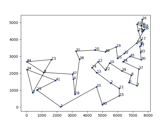
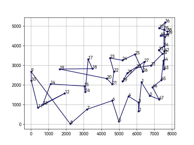
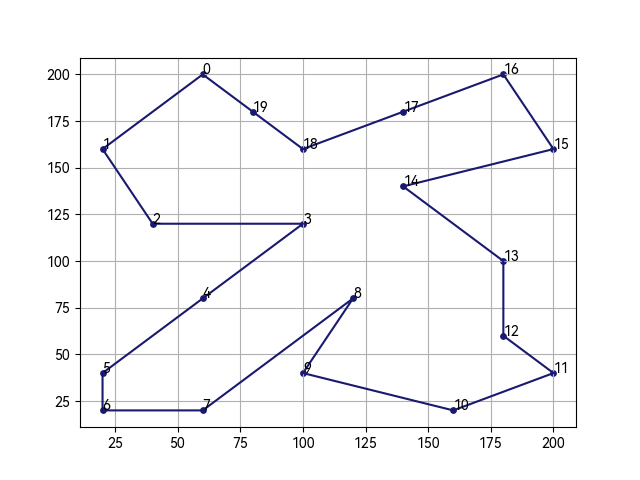
求解结果

运行发现求解效果一般，比遗传算法慢，比蚁群算法求解质量低，程序上如何优化还需要进一步思考。
在python中，I/O密集型任务可以用多线程的方式来实现（threading库）； 然而，对于计算密集型任务，由于python中全局锁GIL的存在，多线程并不能起到一个加速的作用。所以此时，一般使用多进程的方式实现（multiprocessing库）。 我尝试开启多进程，但报错TypeError: cannot pickle 'dict_keys' object。

其他算法求解：

• 基于蚁群算法的TSP问题建模求解（Python）
• 基于模拟退火算法的TSP问题建模求解（Python）

参考文献

1. 基于粒子群算法的无约束优化问题求解

2. 粒子群算法（PSO）求解TSP问题

3. 【建模算法】基于粒子群算法求解TSP问题（Python实现）

4. CVRP问题求解（一）整数编码的粒子群算法
   

5. 利用PSO求解TSP问题

   • Shi X H, Liang Y C, Lee H P, et al. Particle swarm optimization-based algorithms for TSP and generalized TSP[J/OL]. Information Processing Letters, 2007, 103(5): 169-176. https://doi.org/10.1016/j.ipl.2007.03.010.

6. 基于集合的粒子群算法(S-PSO)解决TSP

   • Wei-Neng Chen, Jun Zhang, Chung H S H, et al. A Novel Set-Based Particle Swarm Optimization Method for Discrete Optimization Problems[J/OL]. IEEE Transactions on Evolutionary Computation, 2010, 14(2): 278-300. https://doi.org/10.1109/TEVC.2009.2030331.
   • Gong Y J, Zhang J, Liu O, et al. Optimizing the Vehicle Routing Problem With Time Windows: A Discrete Particle Swarm Optimization Approach[J/OL]. IEEE Transactions on Systems, Man, and Cybernetics, Part C (Applications and Reviews), 2012, 42(2): 254-267. https://doi.org/10.1109/TSMCC.2011.2148712.
   • Kaiwartya O, Kumar S, Lobiyal D K, et al. Multiobjective Dynamic Vehicle Routing Problem and Time Seed Based Solution Using Particle Swarm Optimization[J/OL]. Journal of Sensors, 2015, 2015: 1-14. https://doi.org/10.1155/2015/189832.
   • Yu X, Chen W N, Hu X min, et al. A Set-based Comprehensive Learning Particle Swarm Optimization with Decomposition for Multiobjective Traveling Salesman Problem[C/OL]//Proceedings of the 2015 Annual Conference on Genetic and Evolutionary Computation. Madrid Spain: ACM, 2015: 89-96[2024-01-20]. https://dl.acm.org/doi/10.1145/2739480.2754672.
   • Chen W N, Tan D Z. Set-based discrete particle swarm optimization and its applications: a survey[J/OL]. Frontiers of Computer Science, 2018, 12(2): 203-216. https://doi.org/10.1007/s11704-018-7155-4.