使用scikit-opt中粒子群算法求解约束优化问题

置顶夜来滴星

已于 2024-04-09 13:29:07 修改

阅读量811

点赞数 10

分类专栏： # 智能优化算法文章标签：函数优化不等式约束优化粒子群算法智能优化算法 scikit-opt Python

于 2024-04-09 13:27:40 首次发布

本文链接：https://blog.csdn.net/qq_43276566/article/details/137547190

版权

智能优化算法专栏收录该内容

20 篇文章 3 订阅

订阅专栏

使用scikit-opt中粒子群算法求解函数优化问题

一、有约束情况下的粒子群算法函数寻优思想
二、官网例题求解
三、scikit-opt源码复现

一、有约束情况下的粒子群算法函数寻优思想

粒子群算法求解约束优化问题，关键是约束的处理，初始化将粒子历史最优位置设为 $+\infty$ ，每次迭代若粒子位置满足约束且优于历史最优位置，则更新位置，逐步引导粒子在可行域内搜索最优解。

或者采用罚函数法、增广拉格朗日函数法将约束优化问题转化为无约束优化问题后，可以采用梯度类、粒子群算法进行求解。https://blog.csdn.net/qq_43276566/article/details/136810660

二、官网例题求解

scikit-opt库中，从sko.PSO中导入PSO算法，可以用来求解不等式约束优化问题（目前还不能求解等式约束优化问题），官网例题如下：
$\begin{align} \min & \quad f(x_1, x_2) = -20 \times \text{e}^{-0.2\sqrt{0.5(x_1^2+ x_2^2)}} -\text{e}^{0.5 (\cos 2 \pi x_1 + (\cos 2 \pi x_2))}+20+ \text e \\ \text{s.t.} & \quad (x_1-1)^2 + x_2^2 - 0.5^2 \leq 0 \\ & \quad x_1,x_2 \in [-2,2] \end{align}$
该问题的最优解为 $f (0.95, 0) = 2.58$

官网代码如下：

import numpy as np
import matplotlib.pyplot as plt
from matplotlib.animation import FuncAnimation
from sko.PSO import PSO


def demo_func(x):
    x1, x2 = x
    return -20 * np.exp(-0.2 * np.sqrt(0.5 * (x1 ** 2 + x2 ** 2))) - np.exp(
        0.5 * (np.cos(2 * np.pi * x1) + np.cos(2 * np.pi * x2))) + 20 + np.e


constraint_ueq = (
    lambda x: (x[0] - 1) ** 2 + (x[1] - 0) ** 2 - 0.5 ** 2
    ,
)

max_iter = 50


pso = PSO(func=demo_func, n_dim=2, pop=40, max_iter=max_iter, lb=[-2, -2], ub=[2, 2]
          , constraint_ueq=constraint_ueq, verbose=True)

pso.record_mode = True
pso.run()
print(pso.gbest_y)
print('best_x is ', pso.gbest_x, 'best_y is', pso.gbest_y)

# %% Now Plot the animation


record_value = pso.record_value
X_list, V_list = record_value['X'], record_value['V']

fig, ax = plt.subplots(1, 1)
ax.set_title('title', loc='center')
line = ax.plot([], [], 'b.')

X_grid, Y_grid = np.meshgrid(np.linspace(-2.0, 2.0, 40), np.linspace(-2.0, 2.0, 40))
Z_grid = demo_func((X_grid, Y_grid))
ax.contour(X_grid, Y_grid, Z_grid, 30)

ax.set_xlim(-2, 2)
ax.set_ylim(-2, 2)

t = np.linspace(0, 2 * np.pi, 40)
ax.plot(0.5 * np.cos(t) + 1, 0.5 * np.sin(t), color='r')

plt.ion()
p = plt.show()


def update_scatter(frame):
    i, j = frame // 10, frame % 10
    ax.set_title('iter = ' + str(i))
    X_tmp = X_list[i] + V_list[i] * j / 10.0
    plt.setp(line, 'xdata', X_tmp[:, 0], 'ydata', X_tmp[:, 1])
    return line


ani = FuncAnimation(fig, update_scatter, blit=True, interval=25, frames=max_iter * 10)
plt.show()

ani.save('pso.gif', writer='pillow')

在这里插入图片描述

三、scikit-opt源码复现

scikit-opt有中文文档，并且可以查看源码，遂进行复现：

from matplotlib import cm
from mpl_toolkits.mplot3d import Axes3D
import numpy as np
import matplotlib.pyplot as plt
import matplotlib as mpl

mpl.rcParams['font.sans-serif'] = ['Times New Roman']  # 指定默认字体
mpl.rcParams['axes.unicode_minus'] = False  # 解决保存图像是负号'-'显示为方块的问题


class PSO:
    def __init__(self, function, constraints, lb, ub):
        self.w = 1  # 惯性权重
        self.c1 = 0.5  # 加速系数
        self.c2 = 0.5  # 加速系数
        self.dimension = 2
        self.pop_size = 50
        self.max_iteration = 100

        self.lb = np.array(lb)
        self.ub = np.array(ub)
        assert np.all(self.ub > self.lb), 'upper-bound must be greater than lower-bound'

        self.max_speed = self.ub - self.lb  # 限制粒子的最大速度
        self.function = function
        self.constraints = constraints

    def evaluate(self, X):
        x = X[:, 0]
        y = X[:, 1]
        return self.function(x, y).reshape(-1, 1)

    def check_constraint(self, x):
        # gather all unequal constraint functions
        for constraint_func in self.constraints:
            if constraint_func(x) > 0:
                return False
        return True

    def update_velocity(self, X, V, pbest, gbest):
        """
           根据速度更新公式更新每个粒子的速度
           :param V: 粒子当前的速度矩阵，20*2 的矩阵
           :param X: 粒子当前的位置矩阵，20*2 的矩阵
           :param pbest: 每个粒子历史最优位置，20*2 的矩阵
           :param gbest: 种群历史最优位置，1*2 的矩阵
        """
        r1 = np.random.random(size=(self.pop_size, self.dimension))
        r2 = np.random.random(size=(self.pop_size, self.dimension))
        V = self.w * V + self.c1 * r1 * (pbest - X) + self.c2 * r2 * (gbest - X)  # 直接对照公式写就好了
        return V

    def update_position(self, X, V):
        X = X + V
        X = np.clip(X, self.lb, self.ub)
        return X

    def update_pbest(self, X):
        pass

    def run(self):
        history = []
        # 初始化粒子的位置和速度
        X = np.random.uniform(low=self.lb, high=self.ub, size=(self.pop_size, self.dimension))
        V = np.random.uniform(low=-self.max_speed, high=self.max_speed, size=(self.pop_size, self.dimension))
        pbest_x = X
        pbest_y = np.array([[np.inf]] * self.pop_size)  # pbest_y = Y 不收敛, 必须设置为无穷大
        gbest_x = X[0]
        gbest_y = np.inf

        for i in range(0, self.max_iteration):
            V = self.update_velocity(X, V, pbest_x, gbest_x)  # 更新速度
            X = self.update_position(X, V)  # 更新位置
            Y = self.evaluate(X)  # 计算目标函数值
            # 更新每个粒子的历史最优位置
            need_update = Y < pbest_y
            # print(need_update[0])
            for idx, x in enumerate(X):
                if need_update[idx,]:
                    need_update[idx] = self.check_constraint(x)

            pbest_x = np.where(need_update, X, pbest_x)
            pbest_y = np.where(need_update, Y, pbest_y)

            # 更新群体的最优位置
            idx_min = pbest_y.argmin()
            if gbest_y > pbest_y[idx_min]:
                gbest_x = pbest_x[idx_min, :].copy()
                gbest_y = pbest_y[idx_min]
            history.append((gbest_x, gbest_y))

        x1, x2 = gbest_x
        print(f'x1={x1:.2f}, x2={x2:.2f} 全局最小值：{np.around(gbest_y, 3)}')
        self.plot_objective_value(history)

    def plot_objective_value(self, history):
        obj_list = [gbest_y for gbest_x, gbest_y in history]
        print(obj_list)
        if obj_list[0] == np.inf:
            i = None
            e = None
            for idx, obj in enumerate(obj_list):
                if obj != np.inf:
                    i = idx
                    e = obj
                    break
            for j in range(i):
                obj_list[j] = e
        plt.figure(figsize=(5, 4))
        plt.plot(np.arange(self.max_iteration), obj_list, color="#191970", linewidth=1.5, alpha=1.)
        plt.grid(True)
        plt.xlabel("iteration")
        plt.ylabel("objective value")
        plt.show()


if __name__ == '__main__':
    def demo_func(x1, x2):
        return -20 * np.exp(-0.2 * np.sqrt(0.5 * (x1 ** 2 + x2 ** 2))) - np.exp(
            0.5 * (np.cos(2 * np.pi * x1) + np.cos(2 * np.pi * x2))) + 20 + np.e


    constraint_ueq = (
        lambda x: (x[0] - 1) ** 2 + (x[1] - 0) ** 2 - 0.5 ** 2
        ,
    )

    pso = PSO(function=demo_func,
              constraints=constraint_ueq,
              lb=[-2, -2],
              ub=[2, 2]
              )
    pso.run()

求解结果为：

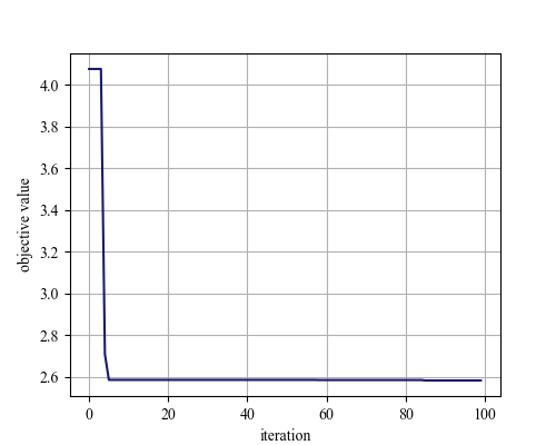
x1=0.94, x2=0.01 全局最小值：[2.583]

目标函数收敛图：
在这里插入图片描述

参考

基于粒子群算法的无约束优化问题求解
Python主要智能优化算法库汇总
https://github.com/guofei9987/scikit-opt/blob/master/examples/demo_pso_ani.py
https://scikit-opt.github.io/scikit-opt/#/zh/README?id=_3-%e7%b2%92%e5%ad%90%e7%be%a4%e7%ae%97%e6%b3%95
使用粒子群算法求解约束优化问题

夜来滴星

关注

10
点赞
踩
21

收藏

觉得还不错? 一键收藏
0
评论
使用scikit-opt中粒子群算法求解约束优化问题

或者采用罚函数法、增广拉格朗日函数法将约束优化问题转化为无约束优化问题后，可以采用梯度类、粒子群算法进行求解。，每次迭代若粒子位置满足约束且优于历史最优位置，则更新位置，逐步引导粒子在可行域内搜索最优解。粒子群算法求解约束优化问题，关键是约束的处理，初始化将粒子历史最优位置设为。
复制链接

扫一扫