YOLOv3-U版解析

论文名称： YOLOv3: An Incremental Improvement

论文下载地址: https://arxiv.org/abs/1804.02767

参考代码: yolov3_spp

YOLOv3 整体网络结构

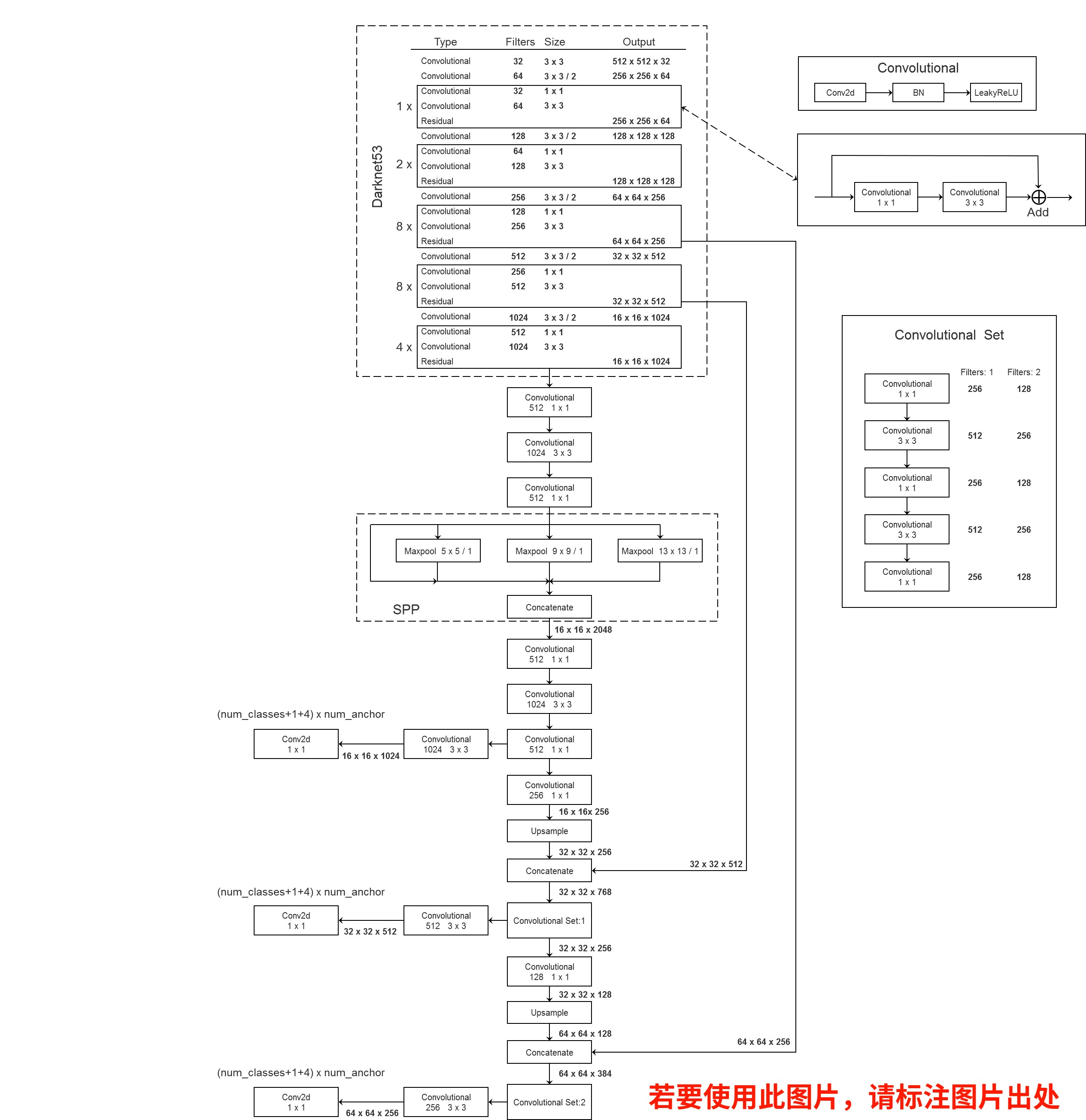
下图是yolov3-SPP的网络结构图，相比于论文的yolov3也有了一些变化，例如网络结构，正负样本匹配方式等，不过这都不是啥大问题，就顺着源码继续学习吧。

网络的Backbone采用的是Darknet-53，此名得益于53个convolutional layers（最后的Connected是全连接层也算卷积层，一共53个）；Neck层采用类似特征金字塔FPN结构；Head采用经典的yoloHead，输出为3个尺度的特征图，分别为13×13、26×26、52×52，对应着9个anchor，每个尺度均分3个anchor, 最后一个维度对应[x,y,w,h,c]和num_class个的one-hot类别标签，以13x13特征图为例，它的shape大小是[B, 3, 13, 13, 4+1+class]

每一层预测anchor的数量对应特征图的大小和分配的anchor模板数量，以13x13特征图为例，数量为13x13x3。

最小的13×13的特征图上由于其感受野最大，应该使用大的anchor(116x90)，(156x198)，(373x326)，这几个坐标是针对原始输入的，因此要除以32把尺度缩放到13×3下使用，适合较大的目标检测。中等特征图26*26适合检测中等目标。52x52的特征图感受野较小，应用最小的anchor box(10x13)，(16x30)，(33x23)，适合检测较小的目标。

图片来源：YOLO v3网络结构分析_yolov3网络结构_太阳花的小绿豆的博客-CSDN博客

预测结果解码

下图展示了目标边界框的回归过程。图中虚线矩形框为Anchor模板宽$p_w$和高$p_h$，实线矩形框为通过网络预测的偏移量(相对Grid Cell的左上角)计算得到的预测边界框，($c_x$,$c_y$)为对应Grid Cell的左上角坐标， ($t_x$,$t_y$,$t_w$,$t_h$)分别为网络预测的边界框中心偏移量以及宽高缩放因子, ($b_x$,$b_y$,$b_w$,$b_h$$)为最终预测的目标边界框。

代码实现:

io = p.clone()  # [bs, anchor, grid, grid, xywh + obj + classes]
io[..., :2] = torch.sigmoid(io[..., :2]) + self.grid  # xy 计算在feature map上的xy坐标
io[..., 2:4] = torch.exp(io[..., 2:4]) * self.anchor_wh  # wh yolo method 计算在feature map上的wh
io[..., :4] *= self.stride  # 换算映射回原图尺度
torch.sigmoid_(io[..., 4:])

正负样本匹配

原版yolov3中正负样本的匹配策略是max iou，对于训练图片中的ground truth，若其中心点落在某个cell内，那么该cell内的3个anchor box负责预测它，具体是哪个anchor box预测它，需要在训练中确定，即由那个与ground truth的IOU最大的anchor box预测它，而剩余的2个anchor box不与该ground truth匹配。

新版中的匹配方法为大于设定阈值即匹配为正样本。

def build_targets(p, targets, model):
    # Build targets for compute_loss(), input targets(image_idx,class,x,y,w,h)
    nt = targets.shape[0]
    tcls, tbox, indices, anch = [], [], [], []
    gain = torch.ones(6, device=targets.device).long()  # normalized to gridspace gain

    multi_gpu = type(model) in (nn.parallel.DataParallel, nn.parallel.DistributedDataParallel)
    for i, j in enumerate(model.yolo_layers):  # j: [89, 101, 113]
        # 获取该yolo predictor对应的anchors
        # 注意anchor_vec是anchors缩放到对应特征层上的尺度
        anchors = model.module.module_list[j].anchor_vec if multi_gpu else model.module_list[j].anchor_vec
        # p[i].shape: [batch_size, 3, grid_h, grid_w, num_params]
        gain[2:] = torch.tensor(p[i].shape)[[3, 2, 3, 2]]  # xyxy gain
        na = anchors.shape[0]  # number of anchors
        # [3] -> [3, 1] -> [3, nt]
        at = torch.arange(na).view(na, 1).repeat(1, nt)  # anchor tensor, same as .repeat_interleave(nt)

        # Match targets to anchors
        a, t, offsets = [], targets * gain, 0
        if nt:  # 如果存在target的话
            # 通过计算anchor模板与所有target的wh_iou来匹配正样本
            # j: [3, nt] , iou_t = 0.20  anchors.shape: [3,2]  给每一个GT分配多个的anchor 由阈值决定
            j = wh_iou(anchors, t[:, 4:6]) > model.hyp['iou_t']  # iou(3,n) = wh_iou(anchors(3,2), gwh(n,2))
            # t.repeat(na, 1, 1): [nt, 6] -> [3, nt, 6]
            # 获取正样本对应的anchor模板与target信息
            a, t = at[j], t.repeat(na, 1, 1)[j]  # filter  a[n]  t[n ,6] n = sum(j)

        # Define
        # long等于to(torch.int64), 数值向下取整
        b, c = t[:, :2].long().T  # image_idx, class
        gxy = t[:, 2:4]  # grid xy
        gwh = t[:, 4:6]  # grid wh
        gij = (gxy - offsets).long()  # 匹配targets所在的grid cell左上角坐标
        gi, gj = gij.T  # grid xy indices

        # Append
        # gain[3]: grid_h, gain[2]: grid_w
        # image_idx, anchor_idx, grid indices(y, x)
        indices.append((b, a, gj.clamp_(0, gain[3]-1), gi.clamp_(0, gain[2]-1)))
        tbox.append(torch.cat((gxy - gij, gwh), 1))  # gt box相对anchor的x,y偏移量以及w,h
        anch.append(anchors[a])  # anchors
        tcls.append(c)  # class
        if c.shape[0]:  # if any targets
            # 目标的标签数值不能大于给定的目标类别数
            assert c.max() < model.nc, 'Model accepts %g classes labeled from 0-%g, however you labelled a class %g. ' \
                                       'See https://github.com/ultralytics/yolov3/wiki/Train-Custom-Data' % (
                                           model.nc, model.nc - 1, c.max())

    return tcls, tbox, indices, anch

损失函数的计算

YOLOv3的损失函数主要分为三个部分：目标定位偏移量损失(只有正样本，GIOU），目标置信度损失（正负样本都参与，BCELoss | FocalLos），目标分类损失(只有正样本，BCELoss | FocalLoss）。

def compute_loss(p, targets, model):  # predictions, targets, model
    device = p[0].device
    lcls = torch.zeros(1, device=device)  # Tensor(0)
    lbox = torch.zeros(1, device=device)  # Tensor(0)
    lobj = torch.zeros(1, device=device)  # Tensor(0)
    tcls, tbox, indices, anchors = build_targets(p, targets, model)  # targets
    h = model.hyp  # hyperparameters
    red = 'mean'  # Loss reduction (sum or mean)

    # Define criteria
    BCEcls = nn.BCEWithLogitsLoss(pos_weight=torch.tensor([h['cls_pw']], device=device), reduction=red)
    BCEobj = nn.BCEWithLogitsLoss(pos_weight=torch.tensor([h['obj_pw']], device=device), reduction=red)

    # class label smoothing https://arxiv.org/pdf/1902.04103.pdf eqn 3
    cp, cn = smooth_BCE(eps=0.0)

    # focal loss
    g = h['fl_gamma']  # focal loss gamma
    if g > 0:
        BCEcls, BCEobj = FocalLoss(BCEcls, g), FocalLoss(BCEobj, g)

    # per output
    for i, pi in enumerate(p):  # layer index, layer predictions
        b, a, gj, gi = indices[i]  # image_idx, anchor_idx, grid_y, grid_x
        tobj = torch.zeros_like(pi[..., 0], device=device)  # target obj

        nb = b.shape[0]  # number of positive samples
        if nb:
            # 对应匹配到正样本的预测信息
            ps = pi[b, a, gj, gi]  # prediction subset corresponding to targets

            # GIoU
            pxy = ps[:, :2].sigmoid()
            pwh = ps[:, 2:4].exp().clamp(max=1E3) * anchors[i]
            pbox = torch.cat((pxy, pwh), 1)  # predicted box
            giou = bbox_iou(pbox.t(), tbox[i], x1y1x2y2=False, GIoU=True)  # giou(prediction, target)
            lbox += (1.0 - giou).mean()  # giou loss

            # Obj
            tobj[b, a, gj, gi] = (1.0 - model.gr) + model.gr * giou.detach().clamp(0).type(tobj.dtype)  # giou ratio

            # Class
            if model.nc > 1:  # cls loss (only if multiple classes)
                t = torch.full_like(ps[:, 5:], cn, device=device)  # targets
                t[range(nb), tcls[i]] = cp
                lcls += BCEcls(ps[:, 5:], t)  # BCE

            # Append targets to text file
            # with open('targets.txt', 'a') as file:
            #     [file.write('%11.5g ' * 4 % tuple(x) + '\n') for x in torch.cat((txy[i], twh[i]), 1)]

        lobj += BCEobj(pi[..., 4], tobj)  # obj loss

    # 乘上每种损失的对应权重
    lbox *= h['giou']
    lobj *= h['obj']
    lcls *= h['cls']

    # loss = lbox + lobj + lcls
    return {"box_loss": lbox,
            "obj_loss": lobj,
            "class_loss": lcls}

小tips

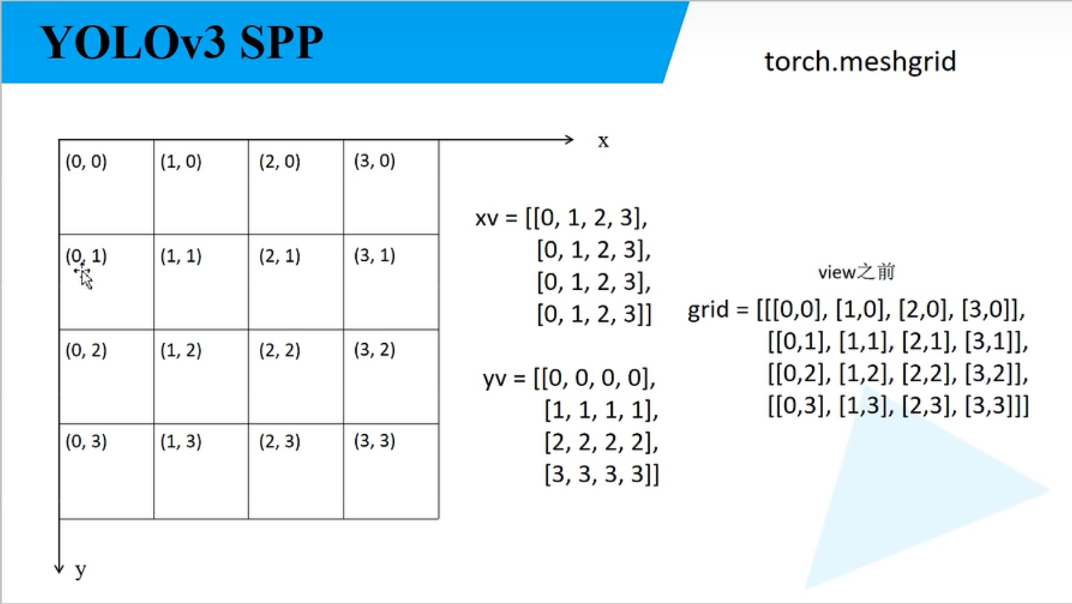
create_grids

self.ny, self.nx = 4  # 特征图大小
# yv [4,4]  xv [4,4]
yv, xv = torch.meshgrid([torch.arange(self.ny, device=device),
                         torch.arange(self.nx, device=device)])
# torch.stack((xv, yv), 2) => [4, 4, 2]
# batch_size, na, grid_h, grid_w, wh
self.grid = torch.stack((xv, yv), 2).view((1, 1, self.ny, self.nx, 2)).float()

广播机制的用法

通过计算anchor模板与所有target的wh_iou来匹配正样本（粗略计算，左上角对齐算IOU），但是巧妙使用了广播机制。

def wh_iou(wh1, wh2):
    # Returns the nxm IoU matrix. wh1 is nx2, wh2 is mx2
    wh1 = wh1[:, None]  # [N,1,2]
    wh2 = wh2[None]  # [1,M,2]
    # 在1维复制M份， 在0维复制N份 取最小
    inter = torch.min(wh1, wh2).prod(2)  # [N,M]  prod(2)在第二个维度上相乘
    return inter / (wh1.prod(2) + wh2.prod(2) - inter)  # iou = inter / (area1 + area2 - inter)