


基于LSTM的城市轨道交通客流量预测
LSTM理论部分
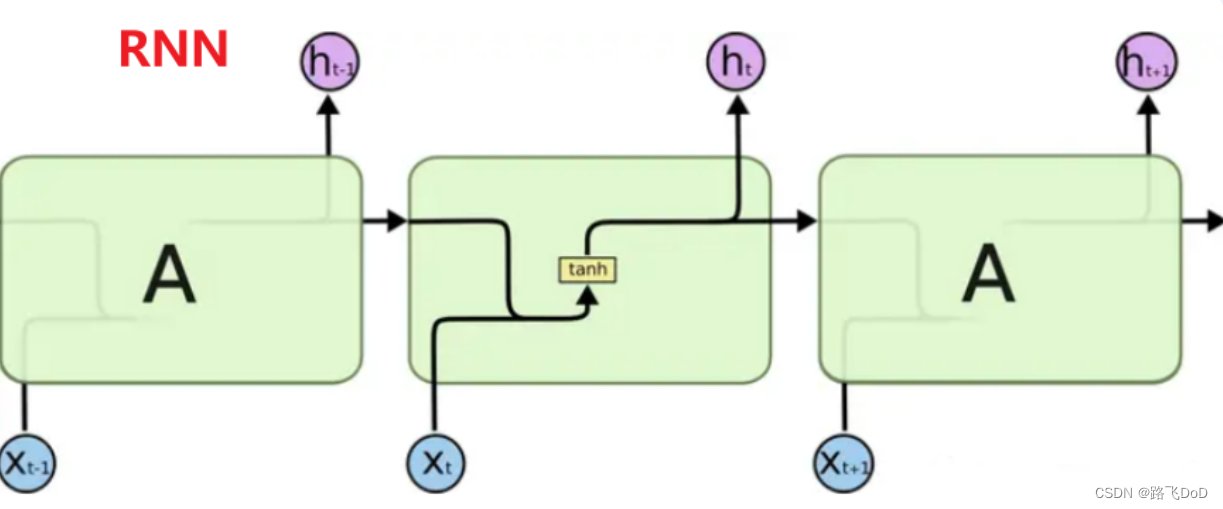
与RNN比较
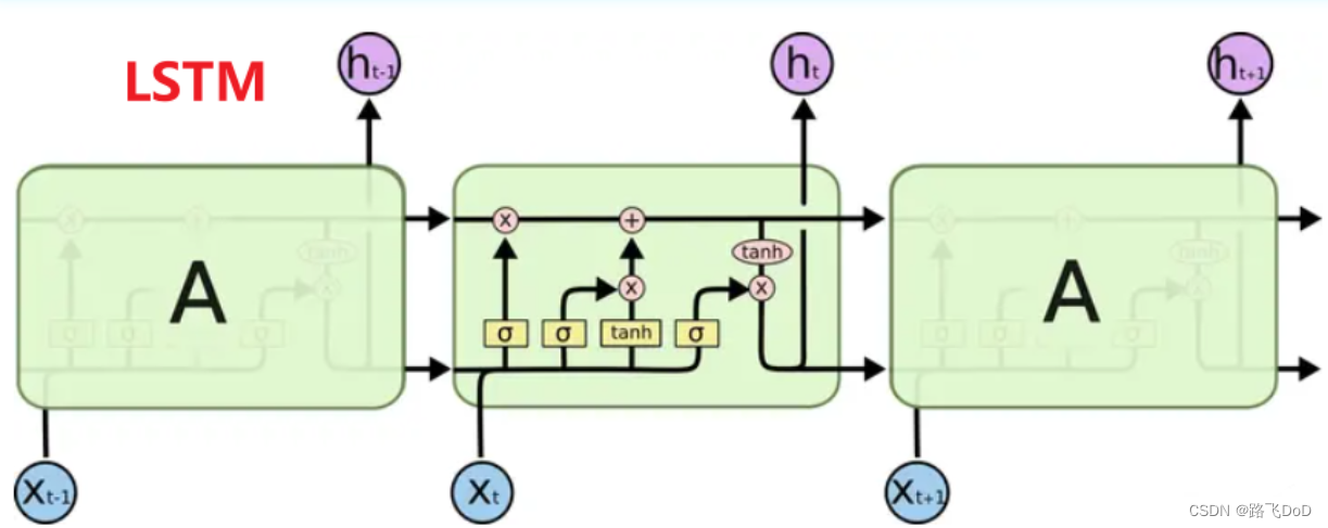
RNN单元在面对长序列数据时,很容易便遭遇梯度弥散,使得RNN只具备短期记忆,即RNN面对长序列数据,仅可获取较近的序列的信息,而对较早期的序列不具备记忆功能,从而丢失信息。为此,为解决该类问题,便提出了LSTM结构,其核心关键在于:
- 提出了门机制:遗忘门、输入门、输出门;
- 细胞状态:在RNN中只有隐藏状态的传播,而在LSTM中,引入了细胞状态。
长短期记忆网络(通常简称为“LSTM”)是一种特殊的 RNN,能够学习长期依赖性。它们由Hochreiter & Schmidhuber (1997)提出,并在后续工作中被许多人完善和推广。它们在解决各种各样的问题上都表现得非常好,并且现在被广泛使用。
LSTM 的设计明确是为了避免长期依赖问题。长时间记住信息实际上是他们的默认行为,而不是他们努力学习的东西!
所有循环神经网络都具有神经网络重复模块链的形式。在标准 RNN 中,这个重复模块将具有非常简单的结构,例如单个 tanh 层。
LSTM 也具有这种链式结构,但重复模块具有不同的结构。神经网络层不是单一的,而是四个,以非常特殊的方式相互作用。
数据集介绍
BRT数据集
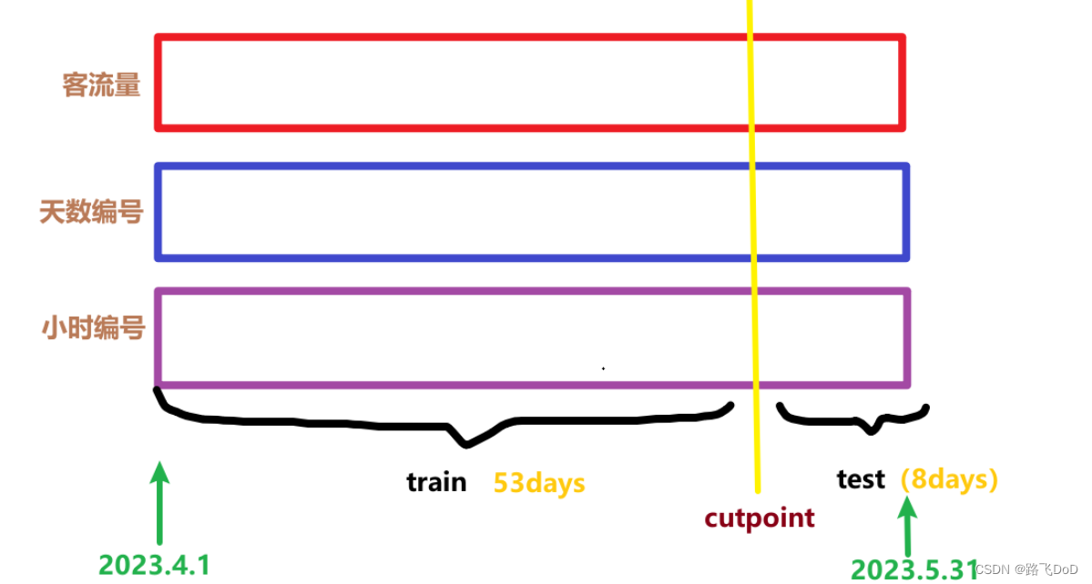
数据集规模:(1464, 45, 1)
本数据集记录了2023年4~5月xiamenBRT45个站点的客流量(按小时划分,61d=61*24=1464h)。
数据粒度:hours。
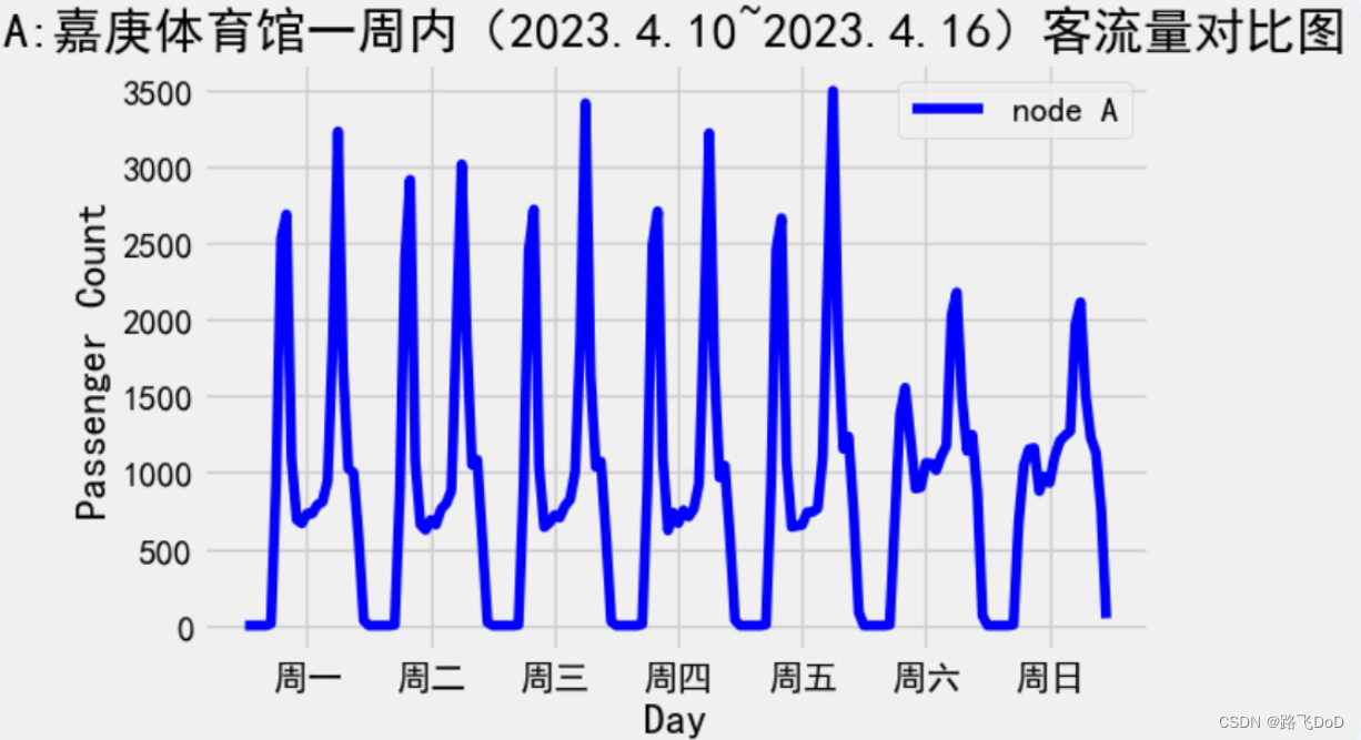
问题定义:基于过去7天的客流量数据预测未来1天的客流量数据。
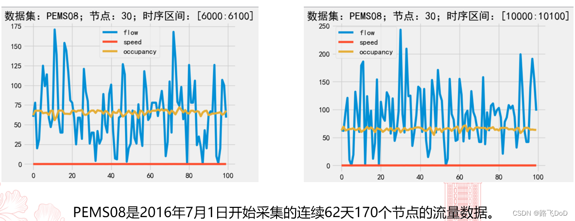
PEMS数据集

数据集预处理
数据集划分
min-max 归一化
这里选择[-1, 1]
def min_max_normalise_tensor(x):
    # shape: [samples, sequence_length, features]
    min_vals = x.min(dim=1).values.unsqueeze(1)
    max_vals = x.max(dim=1).values.unsqueeze(1)
    # data ->[-1, 1]
    normalise_x = 2 * (x - min_vals) / (max_vals - min_vals) - 1
    return normalise_x, min_vals, max_vals

def inverse_min_max_normalise_tensor(x, min_vals, max_vals):
    min_vals = torch.tensor(min_vals).to(device)
    max_vals = torch.tensor(max_vals).to(device)
    # shape: [1, features] -> [1, 1, features]
    min_vals = min_vals.unsqueeze(0)
    max_vals = max_vals.repeat(x.shape[0], 1, 1)
    # [1, 1, features] -> [samples, 1, features]
    min_vals = min_vals.repeat(x.shape[0], 1, 1)
    max_vals = max_vals.repeat(x.shape[0], 1, 1)

    x = (x + 1) / 2 * (max_vals - min_vals) + min_vals
    return x
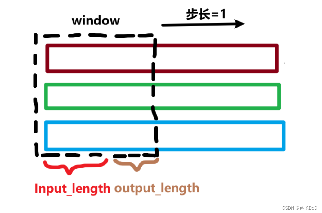
滑动窗口法批次划分数据集
	'''
        input_data  模型输入 连续 input_length  // 24 = 7天的数据
        output_data 模型输出 未来 output_length // 24 = 1天的数据
    '''
    input_data = []
    output_data = []

    # 滑动窗口法
    for i in range(len(train_data) - input_length - output_length + 1):
        input_seq = train_data[i : i + input_length]
        output_seq = train_data[i + input_length : i + input_length + output_length, 0]
        input_data.append(input_seq)
        output_data.append(output_seq)
Input_length:模型输入的序列长度;
output_length:模型输出的序列长度;
这里个人臆想的将模型定性为历史7天(7*24hours)作为input_length,预测未来一天(1*24hours)作为output_length。
代码实现
项目代码结构

模型实现
CNN
import torch.nn as nn

class CNNmodel(nn.Module):
    def __init__(self, input_size, hidden_size, output_size, output_length=1*24) -> None:
        super().__init__()
        self.output_length = output_length
        self.conv = nn.Conv1d(in_channels=input_size, out_channels=hidden_size, kernel_size=3, stride=1, padding=1)
        self.fc = nn.Sequential(
            nn.Linear(hidden_size, hidden_size),
            nn.ReLU(),
            nn.Linear(hidden_size, output_size),
        )
        self.relu = nn.ReLU()

    def forward(self, x):
        # 输入数据形状为(samples, sequence_length, features)
        x = x.permute(0, 2, 1)  # (samples, sequence_length, features) -> (samples, features, sequence_length)
        x = self.conv(x)
        x = self.relu(x)
        x = x.permute(0, 2, 1)  # (samples, features, sequence_length) -> (samples, sequence_length, features)
        x = self.fc(x[:, -self.output_length:, :])
        return x
RNN
import torch.nn as nn

class RNNmodel(nn.Module):
    def __init__(self, input_size, hidden_size, num_layers, output_size, output_length=1 * 24, batch_first=True, bidirectional=False):
        super().__init__()
        self.output_length = output_length
        self.rnn = nn.RNN(
            input_size=input_size,
            hidden_size=hidden_size,
            num_layers=num_layers,
            batch_first=batch_first,
            bidirectional=bidirectional
        )
        self.fc1 = nn.Linear(in_features=hidden_size, out_features=hidden_size)
        self.fc2 = nn.Linear(in_features=hidden_size, out_features=output_size)
        self.relu = nn.ReLU()


    def forward(self, x):
        out, _ = self.rnn(x)
        out = self.fc1(out[:, -self.output_length:, :])
        out = self.relu(out)
        out = self.fc2(out)
        return out
LSTM
import torch.nn as nn

class LSTMmodel(nn.Module):
    def __init__(self, input_size, hidden_size, num_layers, output_size, output_length=1*24, batch_first=True, bidirectional=False):
        super().__init__()
        self.output_length=output_length
        self.lstm = nn.LSTM(
            input_size=input_size,
            hidden_size=hidden_size,
            num_layers=num_layers,
            batch_first=batch_first,
            bidirectional=bidirectional
        )
        if(bidirectional==True):    # 双向LSTM,隐状态翻倍
            self.fc = nn.Sequential(
                nn.Linear(2*hidden_size, hidden_size),
                nn.ReLU(),
                nn.Linear(hidden_size, output_size),
            )
        else:
            self.fc = nn.Sequential(
                nn.Linear(hidden_size, hidden_size),
                nn.ReLU(),
                nn.Linear(hidden_size, output_size),
            )

    def forward(self, x):
        out, _ = self.lstm(x)
        out = self.fc(out[:, -self.output_length:, :])
        return out
GRU
import torch.nn as nn

class GRUmodel(nn.Module):
    def __init__(self, input_size, hidden_size, num_layers, output_size, output_length=1*24, batch_first=True, bidirectional=False):
        super().__init__()
        self.output_length=output_length
        self.gru = nn.GRU(
            input_size=input_size,
            hidden_size=hidden_size,
            num_layers=num_layers,
            batch_first=batch_first,
            bidirectional=bidirectional
        )
        self.fc = nn.Sequential(
            nn.Linear(hidden_size, hidden_size),
            nn.ReLU(),
            nn.Linear(hidden_size, output_size),
        )

    def forward(self, x):
        out, _ = self.gru(x)
        out = self.fc(out[:, -self.output_length:, :])
        return out
CNN-LSTM
import torch.nn as nn

class CNN_LSTM_Model(nn.Module):
    def __init__(self, input_size, output_size, output_length=1*24, batch_first=True) -> None:
        super().__init__()
        self.output_length = output_length
        self.conv1 = nn.Conv1d(in_channels=input_size, out_channels=32, kernel_size=3, stride=1, padding=1)
        self.conv2 = nn.Conv1d(in_channels=32, out_channels=32, kernel_size=3, stride=1, padding=1)
        self.maxpool = nn.MaxPool1d(kernel_size=3, stride=1)
        self.lstm = nn.LSTM(input_size=32, hidden_size=64, num_layers=2, batch_first=batch_first)
        self.fc = nn.Linear(in_features=64, out_features=output_size)
        self.relu = nn.ReLU()

    def forward(self, x):
        # 输入数据形状为(samples, sequence_length, features) [B, S, F]
        x = x.permute(0, 2, 1)  # [B, S, F] -> [B, F, S]
        x = self.conv1(x)       # [B, F, S] -> [B, out_channels_1, S]
        x = self.relu(x)
        x = self.maxpool(x)     # [B, out_channels_1, S] -> [B, out_channels_1, S-2]

        x = self.conv2(x)       # [B, out_channels_1, S-2] -> [B, out_channels_2, S-2]
        x = self.relu(x)
        x = self.maxpool(x)     # [B, out_channels_2, S-2] -> [B, out_channels, S-4]

        x = x.permute(0, 2, 1)
        x, _ = self.lstm(x)
        x = self.fc(x[:, -self.output_length:, :])
        return x
Seq2Seq
胡诌!
import torch
import torch.nn as nn

class Encoder(nn.Module):
    def __init__(self, input_size, hidden_size, num_layers):
        super(Encoder, self).__init__()
        self.hidden_size = hidden_size
        self.num_layers = num_layers
        self.lstm = nn.LSTM(input_size, hidden_size, num_layers, batch_first=True)

    def forward(self, x):
        # 初始化隐藏状态和单元状态
        h0 = torch.zeros(self.num_layers, x.size(0), self.hidden_size).to(x.device)
        c0 = torch.zeros(self.num_layers, x.size(0), self.hidden_size).to(x.device)

        # LSTM前向传播
        out, (hidden_state, cell_state) = self.lstm(x, (h0, c0))
        return out, (hidden_state, cell_state)

class Decoder(nn.Module):
    def __init__(self, output_size, hidden_size, num_layers):
        super(Decoder, self).__init__()
        self.hidden_size = hidden_size
        self.num_layers = num_layers
        self.lstm = nn.LSTM(output_size, hidden_size, num_layers, batch_first=True)
        self.fc = nn.Linear(hidden_size, output_size)

    def forward(self, x, hidden_state, cell_state):
        out, (hidden, cell) = self.lstm(x, (hidden_state, cell_state))
        out = self.fc(out)
        return out, (hidden, cell)

class Seq2Seq(nn.Module):
    def __init__(self, encoder, decoder):
        super(Seq2Seq, self).__init__()
        self.encoder = encoder
        self.decoder = decoder

    def forward(self, input_sequence, target_sequence, teacher_forcing_ratio=1):
        encoder_output, (hidden_state, cell_state) = self.encoder(input_sequence)
        # 初始化解码器的输入
        decoder_input = torch.zeros(input_sequence.size(0), 1, target_sequence.size(2)).to(input_sequence.device)
        # decoder_input = torch.randn(input_sequence.size(0), 1, target_sequence.size(2)).to(input_sequence.device)
        # decoder_input = target_sequence[:, 0:1, :]

        # 存储预测结果
        predicted_outputs = []

        # 是否使用教师强制
        use_teacher_forcing = True if torch.rand(1).item() < teacher_forcing_ratio else False

        # 初始化解码器的隐藏状态和细胞状态
        decoder_hidden = hidden_state
        decoder_cell = cell_state

        # 进行解码器的前向传播

        for t in range(target_sequence.size(1)):
            decoder_output, (decoder_hidden, decoder_cell) = self.decoder(decoder_input, decoder_hidden, decoder_cell)
            predicted_outputs.append(decoder_output)

            # 如果使用教师强制,则下一个时间步的解码器输入为真实目标序列;否则使用模型生成的输出
            decoder_input = target_sequence[:, t:t+1, :] if use_teacher_forcing else decoder_output

        # 将预测结果转换为三维张量
        predicted_outputs = torch.cat(predicted_outputs, dim=1)

        return predicted_outputs
模型加载与配置
def cnn(params):
    global lr, epochs, model
    '''超参数加载'''
    input_size = params["input_size"]           # 输入特征数
    hidden_size = params["hidden_size"]         # CNN output_channels
    output_size = params["output_size"]         # 输出特征数
    lr = params["lr"]                           # 学习率
    epochs = params["epochs"]                   # 训练轮数
    model = CNNmodel(input_size, hidden_size, output_size).to(device)

def rnn(params):
    global lr, epochs, model
    '''超参数加载'''
    input_size = params["input_size"]           # 输入特征数
    hidden_size = params["hidden_size"]         # RNN隐藏层神经元数
    num_layers = params["num_layers"]           # RNN层数
    output_size = params["output_size"]         # 输出特征数
    bidirectional = params["bidirectional"].lower() == "true"   # 是否双向
    lr = params["lr"]                           # 学习率
    epochs = params["epochs"]                   # 训练轮数
    model = RNNmodel(input_size, hidden_size, num_layers, output_size, bidirectional=bidirectional).to(device)

def lstm(params):
    global lr, epochs, model
    '''超参数加载'''
    input_size = params["input_size"]               # 输入特征数
    hidden_size = params["hidden_size"]             # LSTM隐藏层神经元数
    num_layers = params["num_layers"]               # LSTM层数
    bidirectional = params["bidirectional"].lower() == "true"   # 是否双向
    output_size = params["output_size"]             # 输出特征数
    lr = params["lr"]                               # 学习率
    epochs = params["epochs"]                       # 训练轮数

    model = LSTMmodel(input_size, hidden_size, num_layers, output_size, bidirectional=bidirectional).to(device)

def cnn_lstm(params):
    global lr, epochs, model
    '''超参数加载'''
    input_size = params["input_size"]           # 输入特征数
    output_size = params["output_size"]         # 输出特征数
    lr = params["lr"]                           # 学习率
    epochs = params["epochs"]                   # 训练轮数
    model = CNN_LSTM_Model(input_size=input_size, output_size=output_size).to(device)

def gru(params):
    global lr, epochs, model
    '''超参数加载'''
    input_size = params["input_size"]               # 输入特征数
    hidden_size = params["hidden_size"]             # LSTM隐藏层神经元数
    num_layers = params["num_layers"]               # LSTM层数
    bidirectional = params["bidirectional"].lower() == "true"   # 是否双向
    output_size = params["output_size"]             # 输出特征数
    lr = params["lr"]                               # 学习率
    epochs = params["epochs"]                       # 训练轮数
    model = GRUmodel(input_size, hidden_size, num_layers, output_size, bidirectional=bidirectional).to(device)

def attention_lstm(params):
    global lr, epochs, model
    '''超参数加载'''
    input_size = params["input_size"]               # 输入特征数
    hidden_size = params["hidden_size"]             # LSTM隐藏层神经元数
    num_layers = params["num_layers"]               # LSTM层数
    bidirectional = params["bidirectional"].lower() == "true"   # 是否双向
    output_size = params["output_size"]             # 输出特征数
    lr = params["lr"]                               # 学习率
    epochs = params["epochs"]                       # 训练轮数
    model = AttentionLSTMmodel(input_size, hidden_size, num_layers, output_size, bidirectional=bidirectional).to(device)

def seq2seq(params):
    global lr, epochs, model
    '''超参数加载'''
    input_size = params["input_size"]               # 输入特征数
    hidden_size = params["hidden_size"]             # LSTM隐藏层神经元数
    num_layers = params["num_layers"]               # LSTM层数
    output_size = params["output_size"]             # 输出特征数
    lr = params["lr"]                               # 学习率
    epochs = params["epochs"]                       # 训练轮数
    encoder = Encoder(input_size=input_size, hidden_size=hidden_size, num_layers=num_layers).to(device)
    decoder = Decoder(output_size=output_size, hidden_size=hidden_size, num_layers=num_layers).to(device)
    model = Seq2Seq(encoder, decoder).to(device)
训练部分
def train(model_name, save_mod=False):
loss_function = nn.MSELoss()
optimizer = torch.optim.Adam(model.parameters(), lr=lr)
loss_list = [] # 保存训练过程中loss数据
# 开始计时
start_time = time.time() # 记录模型训练开始时间
# train model
for epoch in range(epochs):
optimizer.zero_grad() # 在每个epoch开始时清零梯度
if(model_name=="SEQ2SEQ"):
Y_hat = model(X,Y,1)
else:
Y_hat = model(X)
# print('Y_hat.size: [{},{},{}]'.format(Y_hat.size(0), Y_hat.size(1), Y_hat.size(2)))
# print('Y.size: [{},{},{}]'.format(Y.size(0), Y.size(1), Y.size(2)))
loss = loss_function(Y_hat, Y)
loss.backward()
nn.utils.clip_grad_norm_(parameters=model.parameters(), max_norm=4, norm_type=2)
optimizer.step()
print(f'Epoch [{epoch+1}/{epochs}], MSE-Loss: {loss.item()}')
loss_list.append(loss.item())
end_time = time.time() # 记录模型训练结束时间
total_time = end_time - start_time # 计算总耗时
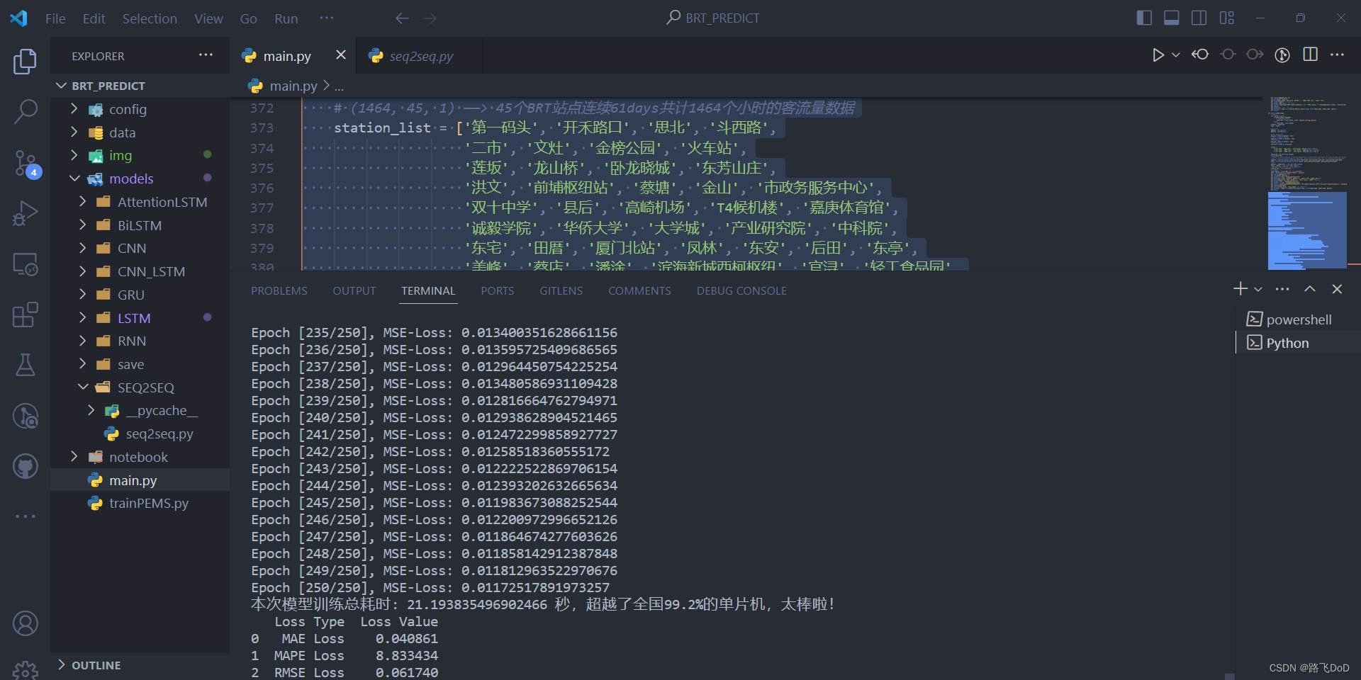
print(f"本次模型训练总耗时: {total_time} 秒,超越了全国99.2%的单片机,太棒啦!")
if save_mod == True:
# save model -> ./**/model_name_eopch{n}.pth
torch.save(model.state_dict(), '{}/{}_epoch{}.pth'.format(save_mod_dir, model_name, epochs))
print("Trained Model have saved in:", '{}/{}_epoch{}.pth'.format(save_mod_dir, model_name, epochs))
# save training loss graph
epoch_index = list(range(1,epochs+1))
plt.figure(figsize=(10, 6))
sns.set(style='darkgrid')
plt.plot(epoch_index, loss_list, marker='.', label='MSE Loss', color='red')
plt.xlabel('Epoch') # x 轴标签
plt.ylabel('MSE Loss') # y 轴标签
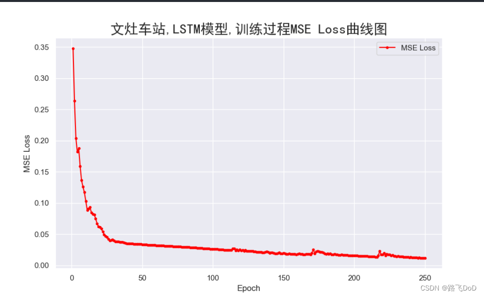
plt.title(f'{data_name}车站,{model_name}模型,训练过程MSE Loss曲线图',fontproperties='SimHei', fontsize=20)
plt.legend()
plt.grid(True) # 添加网格背景
plt.savefig('./img/{}_{}_training_MSEloss_epoch{}.png'.format(data_name, model_name, epochs))
plt.close()
预测部分
def predict(model_name):
# predict
with torch.no_grad():
if(model_name=="SEQ2SEQ"):
# 关闭教师强制策略
testY_hat = model(testX, testY, teacher_forcing_ratio=0)
else:
testY_hat = model(testX)
predict = testY_hat
real = testY
# cal_loss
MAEloss = nn.L1Loss()
MSEloss = nn.MSELoss()
# MAE: 平均绝对误差
mae_val = MAEloss(predict, real)
# MAPE: 平均绝对百分比误差
mape_val = MAPELoss(predict, real)
# MSE:均方误差
mse_val = MSEloss(predict, real)
# RMSE:均方根误差
rmse_val = torch.sqrt(mse_val)
losses = [
{'Loss Type': 'MAE Loss', 'Loss Value': mae_val.cpu().item()},
{'Loss Type': 'MAPE Loss', 'Loss Value': mape_val.cpu().item()},
{'Loss Type': 'RMSE Loss', 'Loss Value': rmse_val.cpu().item()}
]
losses_df = pd.DataFrame(losses)
print(losses_df)
# predict = inverse_min_max_normalise_numpy(predict, min_vals=min_test_data[:,0], max_vals=max_test_data[:,0])
# real = inverse_min_max_normalise_numpy(real, min_vals=min_test_data[:,0], max_vals=max_test_data[:,0])
predict = inverse_min_max_normalise_tensor(testY_hat, min_vals=min_test_data, max_vals=max_test_data)
real = inverse_min_max_normalise_tensor(testY, min_vals=min_test_data, max_vals=max_test_data)
# draw
predict = predict[0, :, 0].cpu().data.numpy()
real = real[0, :, 0].cpu().data.numpy()
# 生成时间序列,时间间隔为1小时,共24小时
time_series = list(range(24))
# 定义时间标签
time_labels = [f"{i}:00" for i in range(24)]
font = FontProperties(family='SimHei', size=20)
plt.figure(figsize=(12, 6))
sns.set(style='darkgrid')
plt.ylabel('客流量', fontproperties=font)
plt.plot(time_series, predict, marker='o', color='red', label='预测值')
plt.plot(time_series, real, marker='o', color='blue', label='真实值')
plt.xlabel('时间', fontproperties=font)
plt.ylabel('客流量', fontproperties=font)
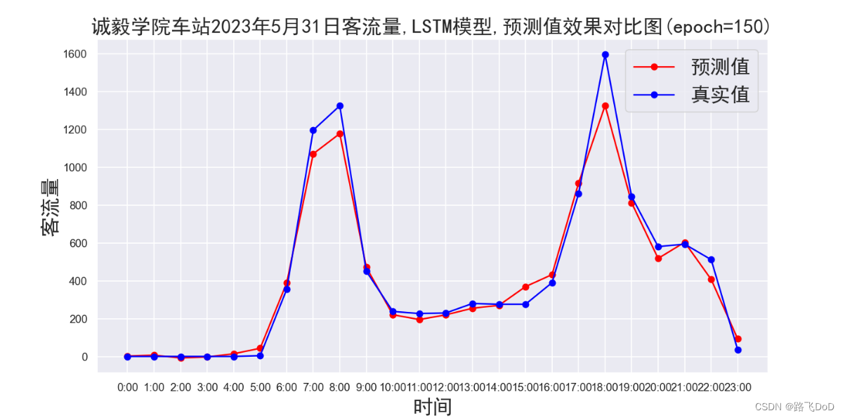
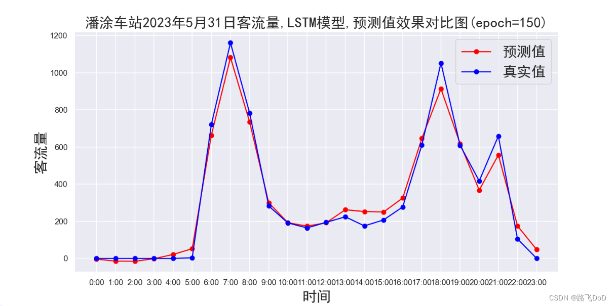
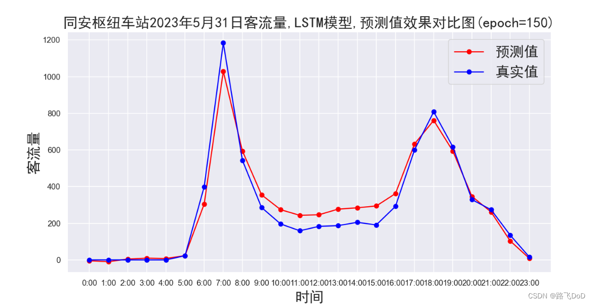
plt.title(f'{data_name}车站2023年5月31日客流量,{model_name}模型,预测值效果对比图(epoch={epochs})', fontproperties=font)
plt.legend(prop=font)
plt.xticks(time_series, time_labels) # 设置时间标签
plt.savefig('./img/{}_{}_prediction_epoch{}.png'.format(data_name, model_name, epochs))
plt.show()
main.py
主要代码在这里。
import torch
import torch.nn as nn
import numpy as np
from models.LSTM.lstm import LSTMmodel
from models.CNN_LSTM.cnn_lstm import CNN_LSTM_Model
from models.RNN.rnn import RNNmodel
from models.CNN.cnn import CNNmodel
from models.GRU.gru import GRUmodel
from models.SEQ2SEQ.seq2seq import Encoder, Decoder, Seq2Seq
from models.AttentionLSTM.attention_lstm import AttentionLSTMmodel
import matplotlib.pyplot as plt
import seaborn as sns
from matplotlib.font_manager import FontProperties
import os
import json
import time
import pandas as pd
os.environ['CUDA_LAUNCH_BLOCKING'] = '1'
device = torch.device("cuda" if torch.cuda.is_available() else "cpu")
X = None
Y = None
testX = None
testY = None
lr = 0.0001
epochs = 100
model = None
min_test_data = None
max_test_data = None                                # 测试集的最大最小值
data_path = "./data/BRT/厦门北站_brtdata.npz"       # 数据集路径
data_name = "厦门北站"                              # 站点数据集名称
save_mod_dir = "./models/save"                      # 模型保存路径

'''load_data'''
def load_data(cut_point, data_path, input_length=7*24, output_length=1*24, days=61, hours=24):
    global min_test_data, max_test_data
    '''
        INPUT:
                cut_point, 训练和测试数据集划分点
                days, 客流数据的总天数
                hours, 每天小时数
                input_length, 模型输入的过去7天的数据作为一个序列
                output_length, 预测未来1天的数据
        OUTPUT:
                train_data
                test_data
    '''
    data = np.load(data_path)['data']
    data = data.astype(np.float32)
    data = data[:, np.newaxis]

    seq_days = np.arange(days)
    seq_hours = np.arange(hours)
    seq_day_hour = np.transpose(
        [np.repeat(seq_days, len(seq_hours)),
         np.tile(seq_hours, len(seq_days))]
    )   # Cartesian Product

    # 按照列方向拼接 --> [客流量, days, hours]
    data = np.concatenate((data, seq_day_hour), axis=1)

    train_data = data[:cut_point]
    test_data = data[cut_point:]

    # 分别进行min-max scaling
    train_data, min_train_data, max_train_data = min_max_normalise_numpy(train_data)
    test_data, min_test_data, max_test_data = min_max_normalise_numpy(test_data)

    '''
        input_data  模型输入 连续 input_length  // 24 = 7天的数据
        output_data 模型输出 未来 output_length // 24 = 1天的数据
    '''
    input_data = []
    output_data = []

    # 滑动窗口法
    for i in range(len(train_data) - input_length - output_length + 1):
        input_seq = train_data[i : i + input_length]
        output_seq = train_data[i + input_length : i + input_length + output_length, 0]
        input_data.append(input_seq)
        output_data.append(output_seq)

    # 转为torch.tensor
    X = torch.tensor(input_data, dtype=torch.float32, device=device)
    Y = torch.tensor(output_data, dtype=torch.float32, device=device)
    Y = Y.unsqueeze(-1)     # 在最后一个维度(维度索引为1)上增加一个维度
    # X = torch.tensor([item.cpu().detach().numpy() for item in input_data], dtype=torch.float32, device=device)
    # Y = torch.tensor([item.cpu().detach().numpy() for item in output_data], dtype=torch.float32, device=device)

    test_inseq = []
    test_outseq = []
    # 滑动窗口法
    for i in range(len(test_data) - input_length - output_length + 1):
        input_seq = test_data[i : i + input_length]
        output_seq = test_data[i + input_length : i + input_length + output_length, 0]

        test_inseq.append(input_seq)
        test_outseq.append(output_seq)

    # 转为torch.tensor
    testX = torch.tensor(test_inseq, dtype=torch.float32, device=device)
    testY = torch.tensor(test_outseq, dtype=torch.float32, device=device)
    testY = testY.unsqueeze(-1)     # 在最后一个维度(维度索引为1)上增加一个维度
    # testX = torch.tensor([item.cpu().detach().numpy() for item in test_inseq], dtype=torch.float32, device=device)
    # testY = torch.tensor([item.cpu().detach().numpy() for item in test_outseq], dtype=torch.float32, device=device)

    # 输出数据形状
    print("数据集处理完毕:")
    print("data - 原数据集 shape:", data.shape)
    print("traindata - Input shape:", X.shape)
    print("traindata - Output shape:", Y.shape)
    print("testdata - Input shape:", testX.shape)
    print("testdata - Output shape:", testY.shape)
    return X, Y, testX, testY

'''min-max Scaling'''
def min_max_normalise_numpy(x):
    # shape: [sequence_length, features]
    min_vals = np.min(x, axis=0)
    max_vals = np.max(x, axis=0)
    # [features] -> shape: [1, features]
    min_vals = np.expand_dims(min_vals, axis=0)
    max_vals = np.expand_dims(max_vals, axis=0)
    # 归一化 -> [-1, 1]
    normalized_data = 2 * (x - min_vals) / (max_vals - min_vals) - 1
    # 归一化 -> [0, 1]
    # normalized_data = (x - min_vals) / (max_vals - min_vals)
    return normalized_data, min_vals, max_vals

def inverse_min_max_normalise_numpy(normalised_x, min_vals, max_vals):
    x = (normalised_x + 1) / 2 * (max_vals - min_vals) + min_vals
    return x

def min_max_normalise_tensor(x):
    # shape: [samples, sequence_length, features]
    min_vals = x.min(dim=1).values.unsqueeze(1)
    max_vals = x.max(dim=1).values.unsqueeze(1)
    # data ->[-1, 1]
    normalise_x = 2 * (x - min_vals) / (max_vals - min_vals) - 1
    return normalise_x, min_vals, max_vals

def inverse_min_max_normalise_tensor(x, min_vals, max_vals):
    min_vals = torch.tensor(min_vals).to(device)
    max_vals = torch.tensor(max_vals).to(device)
    # shape: [1, features] -> [1, 1, features]
    min_vals = min_vals.unsqueeze(0)
    max_vals = max_vals.repeat(x.shape[0], 1, 1)
    # [1, 1, features] -> [samples, 1, features]
    min_vals = min_vals.repeat(x.shape[0], 1, 1)
    max_vals = max_vals.repeat(x.shape[0], 1, 1)

    x = (x + 1) / 2 * (max_vals - min_vals) + min_vals
    return x

# MAPE: 平均绝对百分比误差
def MAPELoss(y_hat, y):
    x = torch.tensor(0.0001, dtype=torch.float32).to(device)
    y_new = torch.where(y==0, x, y)    # 防止分母为0
    abs_error = torch.abs((y - y_hat) / y_new)
    mape = 100. * torch.mean(abs_error)
    return mape

def cnn(params):
    global lr, epochs, model
    '''超参数加载'''
    input_size = params["input_size"]           # 输入特征数
    hidden_size = params["hidden_size"]         # CNN output_channels
    output_size = params["output_size"]         # 输出特征数
    lr = params["lr"]                           # 学习率
    epochs = params["epochs"]                   # 训练轮数
    model = CNNmodel(input_size, hidden_size, output_size).to(device)

def rnn(params):
    global lr, epochs, model
    '''超参数加载'''
    input_size = params["input_size"]           # 输入特征数
    hidden_size = params["hidden_size"]         # RNN隐藏层神经元数
    num_layers = params["num_layers"]           # RNN层数
    output_size = params["output_size"]         # 输出特征数
    bidirectional = params["bidirectional"].lower() == "true"   # 是否双向
    lr = params["lr"]                           # 学习率
    epochs = params["epochs"]                   # 训练轮数
    model = RNNmodel(input_size, hidden_size, num_layers, output_size, bidirectional=bidirectional).to(device)

def lstm(params):
    global lr, epochs, model
    '''超参数加载'''
    input_size = params["input_size"]               # 输入特征数
    hidden_size = params["hidden_size"]             # LSTM隐藏层神经元数
    num_layers = params["num_layers"]               # LSTM层数
    bidirectional = params["bidirectional"].lower() == "true"   # 是否双向
    output_size = params["output_size"]             # 输出特征数
    lr = params["lr"]                               # 学习率
    epochs = params["epochs"]                       # 训练轮数

    model = LSTMmodel(input_size, hidden_size, num_layers, output_size, bidirectional=bidirectional).to(device)

def cnn_lstm(params):
    global lr, epochs, model
    '''超参数加载'''
    input_size = params["input_size"]           # 输入特征数
    output_size = params["output_size"]         # 输出特征数
    lr = params["lr"]                           # 学习率
    epochs = params["epochs"]                   # 训练轮数
    model = CNN_LSTM_Model(input_size=input_size, output_size=output_size).to(device)

def gru(params):
    global lr, epochs, model
    '''超参数加载'''
    input_size = params["input_size"]               # 输入特征数
    hidden_size = params["hidden_size"]             # LSTM隐藏层神经元数
    num_layers = params["num_layers"]               # LSTM层数
    bidirectional = params["bidirectional"].lower() == "true"   # 是否双向
    output_size = params["output_size"]             # 输出特征数
    lr = params["lr"]                               # 学习率
    epochs = params["epochs"]                       # 训练轮数
    model = GRUmodel(input_size, hidden_size, num_layers, output_size, bidirectional=bidirectional).to(device)

def attention_lstm(params):
    global lr, epochs, model
    '''超参数加载'''
    input_size = params["input_size"]               # 输入特征数
    hidden_size = params["hidden_size"]             # LSTM隐藏层神经元数
    num_layers = params["num_layers"]               # LSTM层数
    bidirectional = params["bidirectional"].lower() == "true"   # 是否双向
    output_size = params["output_size"]             # 输出特征数
    lr = params["lr"]                               # 学习率
    epochs = params["epochs"]                       # 训练轮数
    model = AttentionLSTMmodel(input_size, hidden_size, num_layers, output_size, bidirectional=bidirectional).to(device)

def seq2seq(params):
    global lr, epochs, model
    '''超参数加载'''
    input_size = params["input_size"]               # 输入特征数
    hidden_size = params["hidden_size"]             # LSTM隐藏层神经元数
    num_layers = params["num_layers"]               # LSTM层数
    output_size = params["output_size"]             # 输出特征数
    lr = params["lr"]                               # 学习率
    epochs = params["epochs"]                       # 训练轮数
    encoder = Encoder(input_size=input_size, hidden_size=hidden_size, num_layers=num_layers).to(device)
    decoder = Decoder(output_size=output_size, hidden_size=hidden_size, num_layers=num_layers).to(device)
    model = Seq2Seq(encoder, decoder).to(device)

def train(model_name, save_mod=False):
    loss_function = nn.MSELoss()
    optimizer = torch.optim.Adam(model.parameters(), lr=lr)
    loss_list = []      # 保存训练过程中loss数据
    # 开始计时
    start_time = time.time()  # 记录模型训练开始时间

    # train model
    for epoch in range(epochs):
        optimizer.zero_grad()   # 在每个epoch开始时清零梯度
        if(model_name=="SEQ2SEQ"):
            Y_hat = model(X,Y,1)
        else:
            Y_hat = model(X)
        # print('Y_hat.size: [{},{},{}]'.format(Y_hat.size(0), Y_hat.size(1), Y_hat.size(2)))
        # print('Y.size: [{},{},{}]'.format(Y.size(0), Y.size(1), Y.size(2)))
        loss = loss_function(Y_hat, Y)
        loss.backward()
        nn.utils.clip_grad_norm_(parameters=model.parameters(), max_norm=4, norm_type=2)
        optimizer.step()
        print(f'Epoch [{epoch+1}/{epochs}], MSE-Loss: {loss.item()}')
        loss_list.append(loss.item())
    end_time = time.time()  # 记录模型训练结束时间
    total_time = end_time - start_time  # 计算总耗时
    print(f"本次模型训练总耗时: {total_time} 秒,超越了全国99.2%的单片机,太棒啦!")
    if save_mod == True:
        # save model -> ./**/model_name_eopch{n}.pth
        torch.save(model.state_dict(), '{}/{}_epoch{}.pth'.format(save_mod_dir, model_name, epochs))
        print("Trained Model have saved in:", '{}/{}_epoch{}.pth'.format(save_mod_dir, model_name, epochs))

    # save training loss graph
    epoch_index = list(range(1,epochs+1))
    plt.figure(figsize=(10, 6))
    sns.set(style='darkgrid')
    plt.plot(epoch_index, loss_list, marker='.', label='MSE Loss', color='red')
    plt.xlabel('Epoch')  # x 轴标签
    plt.ylabel('MSE Loss')  # y 轴标签
    plt.title(f'{data_name}车站,{model_name}模型,训练过程MSE Loss曲线图',fontproperties='SimHei', fontsize=20)
    plt.legend()
    plt.grid(True)  # 添加网格背景
    plt.savefig('./img/{}_{}_training_MSEloss_epoch{}.png'.format(data_name, model_name, epochs))
    plt.close()

def predict(model_name):
    # predict
    with torch.no_grad():
        if(model_name=="SEQ2SEQ"):
            # 关闭教师强制策略
            testY_hat = model(testX, testY, teacher_forcing_ratio=0)
        else:
            testY_hat = model(testX)
    predict = testY_hat
    real = testY

    # cal_loss
    MAEloss = nn.L1Loss()
    MSEloss = nn.MSELoss()

    # MAE: 平均绝对误差
    mae_val = MAEloss(predict, real)
    # MAPE: 平均绝对百分比误差
    mape_val = MAPELoss(predict, real)
    # MSE:均方误差
    mse_val = MSEloss(predict, real)
    # RMSE:均方根误差
    rmse_val = torch.sqrt(mse_val)

    losses = [
        {'Loss Type': 'MAE Loss', 'Loss Value': mae_val.cpu().item()},
        {'Loss Type': 'MAPE Loss', 'Loss Value': mape_val.cpu().item()},
        {'Loss Type': 'RMSE Loss', 'Loss Value': rmse_val.cpu().item()}
    ]
    losses_df = pd.DataFrame(losses)
    print(losses_df)
    # predict = inverse_min_max_normalise_numpy(predict, min_vals=min_test_data[:,0], max_vals=max_test_data[:,0])
    # real = inverse_min_max_normalise_numpy(real, min_vals=min_test_data[:,0], max_vals=max_test_data[:,0])
    predict = inverse_min_max_normalise_tensor(testY_hat, min_vals=min_test_data, max_vals=max_test_data)
    real = inverse_min_max_normalise_tensor(testY, min_vals=min_test_data, max_vals=max_test_data)
    # draw
    predict = predict[0, :, 0].cpu().data.numpy()
    real = real[0, :, 0].cpu().data.numpy()
    # 生成时间序列,时间间隔为1小时,共24小时
    time_series = list(range(24))
    # 定义时间标签
    time_labels = [f"{i}:00" for i in range(24)]
    font = FontProperties(family='SimHei', size=20)
    plt.figure(figsize=(12, 6))
    sns.set(style='darkgrid')
    plt.ylabel('客流量', fontproperties=font)
    plt.plot(time_series, predict, marker='o', color='red', label='预测值')
    plt.plot(time_series, real, marker='o', color='blue', label='真实值')
    plt.xlabel('时间', fontproperties=font)
    plt.ylabel('客流量', fontproperties=font)
    plt.title(f'{data_name}车站2023年5月31日客流量,{model_name}模型,预测值效果对比图(epoch={epochs})', fontproperties=font)
    plt.legend(prop=font)
    plt.xticks(time_series, time_labels)  # 设置时间标签
    plt.savefig('./img/{}_{}_prediction_epoch{}.png'.format(data_name, model_name, epochs))
    plt.show()

def main(model_name, save_mod):
    '''加载数据集'''
    global X, Y, testX, testY
    X, Y, testX, testY = load_data(cut_point=1272, data_path=data_path)

    '''读取超参数配置文件'''
    params = None
    with open(f"./config/{model_name.lower()}_params.json", 'r', encoding='utf-8') as file:
        params = json.load(file)

    if model_name == "RNN":
        rnn(params)
    elif model_name == "LSTM":
        lstm(params)
    elif model_name == "CNN_LSTM":
        cnn_lstm(params)
    elif model_name == "GRU":
        gru(params)
    elif model_name == "CNN":
        cnn(params)
    elif model_name == "Attention_LSTM":
        attention_lstm(params)
    elif model_name == "SEQ2SEQ":
        seq2seq(params)

    train(model_name=model_name, save_mod=save_mod)
    predict(model_name=model_name)

if __name__ == '__main__':
    '''CHOOSE DATAPATH'''
    # (1464, 45, 1) ——> 45个BRT站点连续61days共计1464个小时的客流量数据
    station_list = ['第一码头', '开禾路口', '思北', '斗西路',
                    '二市', '文灶', '金榜公园', '火车站',
                    '莲坂', '龙山桥', '卧龙晓城', '东芳山庄',
                    '洪文', '前埔枢纽站', '蔡塘', '金山', '市政务服务中心',
                    '双十中学', '县后', '高崎机场', 'T4候机楼', '嘉庚体育馆',
                    '诚毅学院', '华侨大学', '大学城', '产业研究院', '中科院',
                    '东宅', '田厝', '厦门北站', '凤林', '东安', '后田', '东亭',
                    '美峰', '蔡店', '潘涂', '滨海新城西柯枢纽', '官浔', '轻工食品园',
                    '四口圳', '工业集中区', '第三医院', '城南', '同安枢纽']
    # 创建一个字典,将数字与车站名称进行映射
    station_dict = {i: station_list[i-1] for i in range(1, len(station_list)+1)}
    # 创建 DataFrame
    df = pd.DataFrame(list(station_dict.items()), columns=['编号', '车站名称'])
    # 设置显示宽度以保持对齐
    pd.set_option('display.max_colwidth', 28)
    print(df.to_string(index=False))
    user_input = input("请输入你要训练的车站数据集编号(1~45,否则随机选择):")
    if int(user_input) in station_dict:
        data_name = station_dict[int(user_input)]
    else:
        # 随机选择一个站点(1-45之间的一个站点)
        random_station = np.random.randint(1, 46)
        data_name = station_list[random_station]
    data_path = f"./data/BRT/{data_name}_brtdata.npz"
    print("数据加载中, 请稍后……", data_path)

    '''INPUT YOUR MODEL NAME'''
    name_list = ["CNN", "RNN", "LSTM", "CNN_LSTM", "GRU", "Attention_LSTM", "SEQ2SEQ"]
    model_name = input("请输入要使用的模型【1: CNN   2: RNN   3: LSTM   4: CNN_LSTM   5: GRU   6: Attention_LSTM   7: SEQ2SEQ】\n")
    if model_name.isnumeric() and int(model_name) <= len(name_list):
        model_name = name_list[int(model_name) - 1]
    '''SAVE MODE'''
    save_mod = input("是否要保存训练后的模型?(输入 '1' 保存,否则不保存)\n")
    if int(save_mod) == 1:
        save_mod = True
    else:
        save_mod = False
    '''main()'''
    main(model_name, save_mod)
启动!!!
可以看到,我们的数据集规模还是比较小的,使用GPU训练,21秒即跑完全程,最终模型评估采用MAE、MAPE、RMSE。
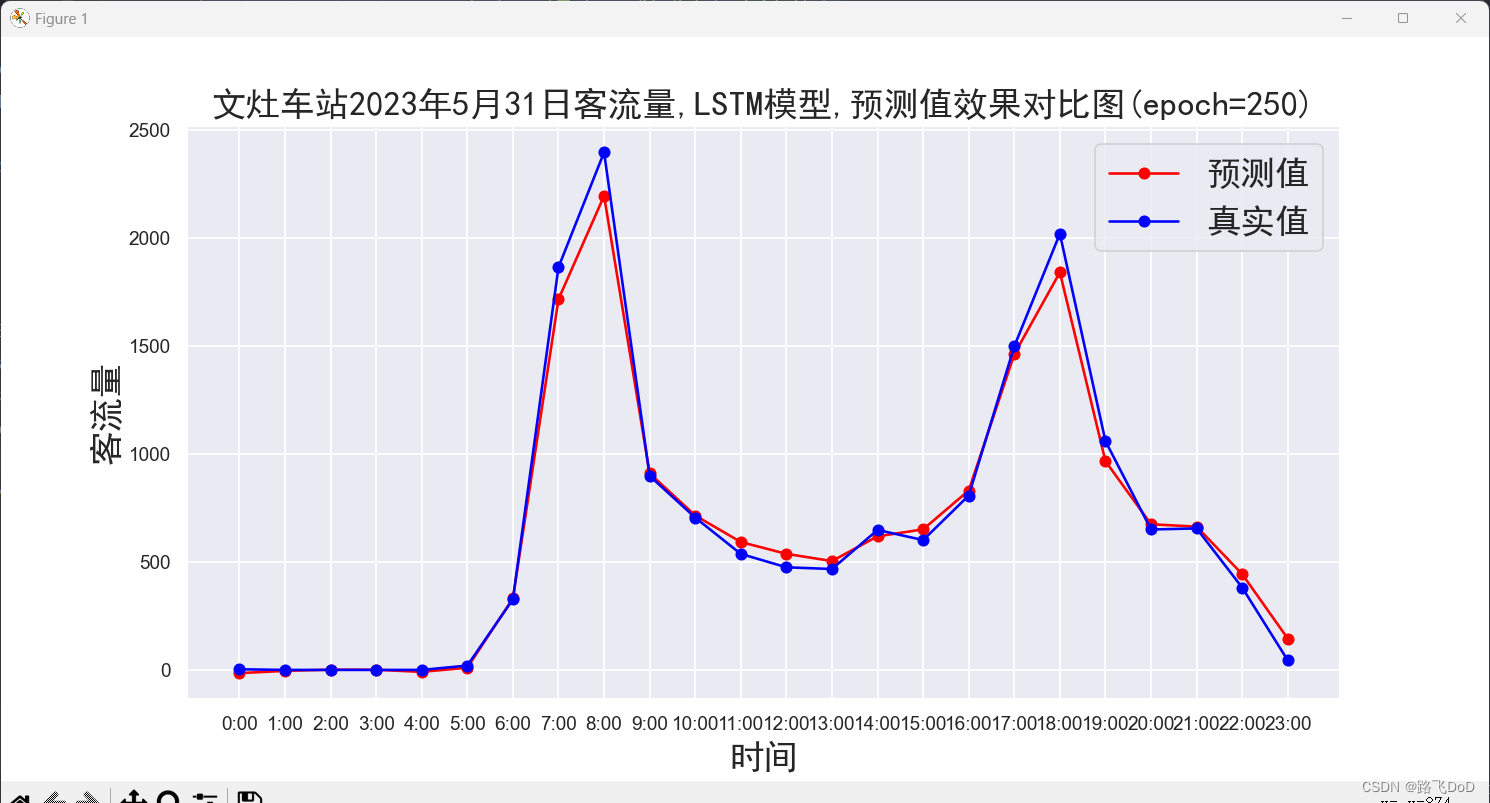
BRT数据集预测结果可视化
😁😁😁
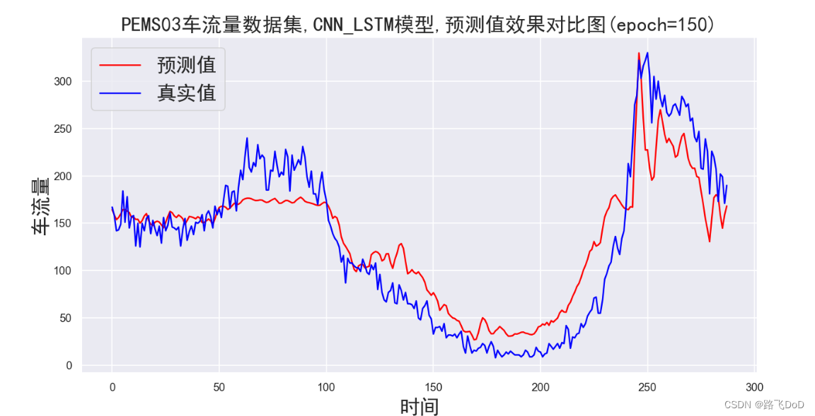
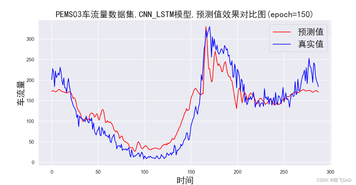
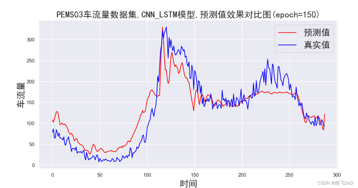
PEMS03数据集预测结果可视化
😥😥😥
Bi-LSTM对照
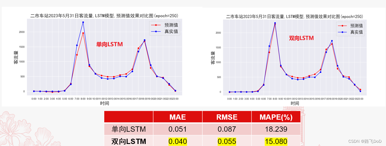
模型横向对比

Git源码🏃
Git Push error: OpenSSL SSL_read: Connection was reset, errno 10054
如果你开启了VPN,很可能是因为代理的问题,这时候设置一下http.proxy就可以了。
一定要查看自己的VPN端口号,假如你的端口号是7890,在git bash命令行中输入以下命令即可:
git config --global http.proxy 127.0.0.1:7890
git config --global https.proxy 127.0.0.1:7890
下面是几个常用的git配置查看命令:
git config --global http.proxy # 查看git的http代理配置
git config --global https.proxy # 查看git的https代理配置
git config --global -l # 查看git的所有配置


 859
859

 被折叠的 条评论
为什么被折叠?
被折叠的 条评论
为什么被折叠?
 到【灌水乐园】发言


