图像分类入门（六）

EfficientNet V2

EfficientNetV1中，关注的更多是模型的Flops，产生了一系列问题。

• 训练图像尺寸过大时，训练速度过慢。
• 在网络浅层中使用Depthwise convolutions速度会很慢
• 同等的放大每个stage是次优的（即简单地增加网络的深度、宽度或输入分辨率并不能同时保证模型的准确性和效率。）

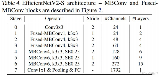
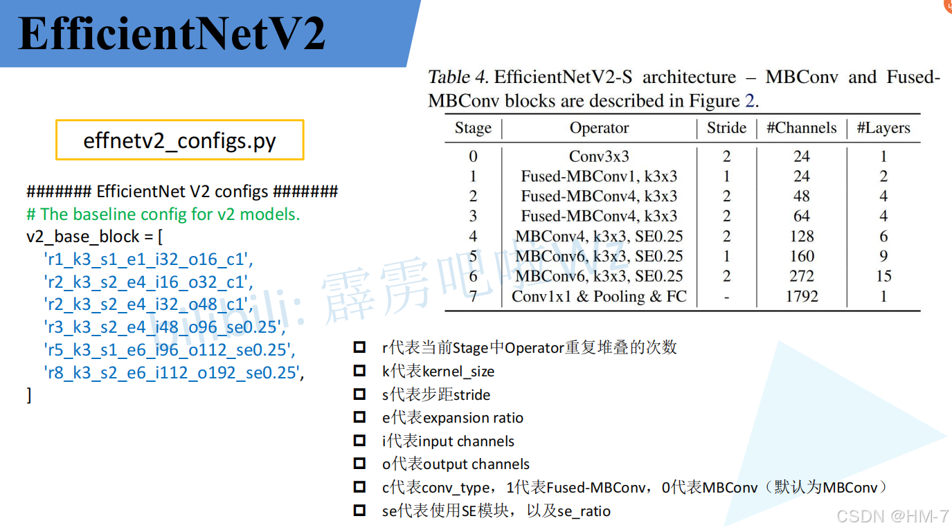
网络框架

• 除了使用MBConv模块，还使用Fused-MBConv模块
• 会使用较小的expansion ratio
• 偏向使用更小的kernel_size(3x3)
• 移除了EfficientNetV1中最后一个步距为1的stage（V1中
  的stage8）
  

Fused-MBConv模块

在网络浅层中使用Depthwise convolutions速度会很慢。无法充分利用现有的一
些加速器（虽然理论上计算量很小，但实际使用起来并没有想象中那么快）。
故引入Fused-MBConv结构。

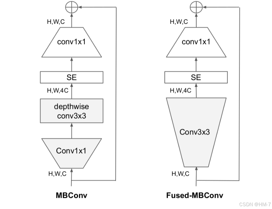
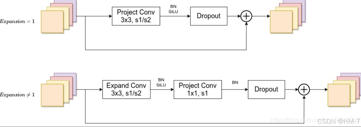
结构相较于MBConv，减少了一开始的1x1的升维卷积和3x3的DW卷积，取而代之的是3x3的普通卷积。当Expansion为1时，仅有一个3x3的升维卷积，不为一时为expand3x3卷积和1x1的升维卷积。
这里的Expansion即为结构图中conv后的数字即expand_ratio。

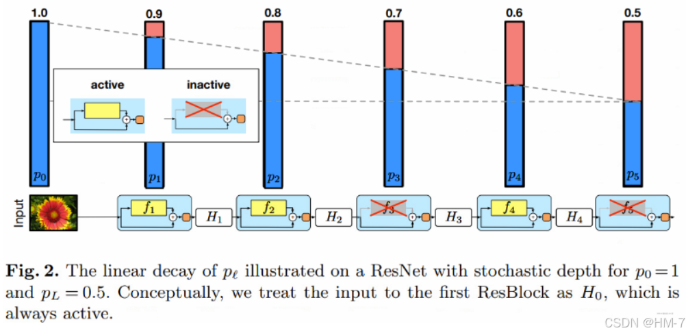
随机深度

具有残差块的网络训练时间过久，为了解决此问题，引入了随机深度的技术。即在我们可以在训练过程中任意地丢弃一些层，并在测试过程中使用完整的网络。通常是通过在训练过程中随机地选择网络中的某些层来“激活”或“禁用”，从而改变网络的结构。这种方法可以让网络在每次前向传播时都采用不同的深度，使其在训练中接触到多种网络配置。

基本思想

在训练中，如果一个特定的残差块被启用了，那么它的输入就会同时流经恒等表换shortcut（identity shortcut）和权重层；否则输入就只会流经恒等变换shortcut。

在训练的过程中，每一个层都有一个“生存概率”，并且都会被任意丢弃。在测试过程中，所有的block都将保持被激活状态，而且block都将根据其在训练中的生存概率进行调整。

假设H1是第一个残差块的输出结果。f1是第一个残差块主分支的输出，b1是一个随机变量(只有1或者0，反映一个block是否是被激活的，或者是否启用当前主分支)。那么加了随机深度的Dropout之后的残差块输出公式计算如下：

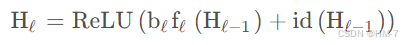
原先的残差结构，即跳跃连接＋主分支后接激活函数，此时仅多了b1来控制主分支是否有效，即block是否激活。若b1=0则：

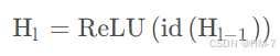
此时即直接走跳跃连接，此时主分支不起作用即当前残差块失活。
作者通过优化公式，且一个“线性衰减规律”应用于每一层的生存概率，他们表示，由于较早的层会提取低级特征，而这些低级特征会被后面的层所利用，所以这些层不应该频繁地被丢弃。这样，最终生成的规则就变成了这样：

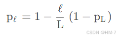
pl表示在l层训练的存活概率，L表示block的数量，PL即输入的dropout_rate，l为第l层的残差块。

具体分析下实现代码：
在droppath函数中：

• 首先进行判断，此时丢弃概率或是否处于训练模式，不符合则退出。
• 计算保留概率keep_prob=1-drop_prob
• 然后根据输入张量的批次大小生成随机张量的形状。创建一个批次维度后跟随大小为 1 的维度，以适应不同形状的张量（例如 2D、3D 等）。
• 创建一个随机张量，其中每个元素均来自均匀分布。这个张量将用于决定是否丢弃某个路径。通过加上 keep_prob，其值范围从 keep_prob 到 1 + keep_prob。
• 使用向下取整操作对张量进行二值化。将大于或等于 1 的值设为 1（活跃路径），小于 1 的值设为 0（丢弃路径）
• 输出通过将输入张量 x 除以 keep_prob（以适当缩放激活值），然后乘以 random_tensor 来计算。这有效地丢弃了某些路径，同时保持整体输出的比例。

def drop_path(x, drop_prob: float = 0., training: bool = False):
    if drop_prob == 0. or not training:
        return x
    keep_prob = 1 - drop_prob
    # 根据输入张量的批次大小生成随机张量的形状。创建一个批次维度后跟随大小为 1 的维度，以适应不同形状的张量（例如 2D、3D 等）。
    shape = (x.shape[0],) + (1,) * (x.ndim - 1)  # work with diff dim tensors, not just 2D ConvNets
    random_tensor = keep_prob + torch.rand(shape, dtype=x.dtype, device=x.device)
    random_tensor.floor_()  # binarize
    output = x.div(keep_prob) * random_tensor
    return output


class DropPath(nn.Module):

    def __init__(self, drop_prob=None):
        super(DropPath, self).__init__()
        self.drop_prob = drop_prob

    def forward(self, x):
        return drop_path(x, self.drop_prob, self.training)

代码实现

Model

与V1中类似，首先定义Dropout的处理函数。

def drop_path(x, drop_prob: float = 0., training: bool = False):
    if drop_prob == 0. or not training:
        return x
    keep_prob = 1 - drop_prob
    # 根据输入张量的批次大小生成随机张量的形状。创建一个批次维度后跟随大小为 1 的维度，以适应不同形状的张量（例如 2D、3D 等）。
    shape = (x.shape[0],) + (1,) * (x.ndim - 1)  # work with diff dim tensors, not just 2D ConvNets
    random_tensor = keep_prob + torch.rand(shape, dtype=x.dtype, device=x.device)
    random_tensor.floor_()  # binarize
    output = x.div(keep_prob) * random_tensor
    return output


class DropPath(nn.Module):

    def __init__(self, drop_prob=None):
        super(DropPath, self).__init__()
        self.drop_prob = drop_prob

    def forward(self, x):
        return drop_path(x, self.drop_prob, self.training)

定义卷积BN激活通用方法和SE模块

class ConvBNAct(nn.Module):
    def __init__(self,
                 in_planes: int,
                 out_planes: int,
                 kernel_size: int = 3,
                 stride: int = 1,
                 groups: int = 1,
                 norm_layer: Optional[Callable[..., nn.Module]] = None,
                 activation_layer: Optional[Callable[..., nn.Module]] = None):
        super(ConvBNAct, self).__init__()
        padding = (kernel_size - 1) // 2
        if norm_layer is None:
            norm_layer = nn.BatchNorm2d
        if activation_layer is None:
            activation_layer = nn.SiLU

        self.conv = nn.Conv2d(in_channels=in_planes,
                              out_channels=out_planes,
                              kernel_size=kernel_size,
                              stride=stride,
                              padding=padding,
                              groups=groups,
                              bias=False)

        self.bn = norm_layer(out_planes)
        self.act = activation_layer()

    def forward(self, x):
        x = self.conv(x)
        x = self.bn(x)
        x = self.act(x)
        return x


class SqueezeExcitation(nn.Module):
    def __init__(self,
                 input_c: int,
                 expand_c: int,
                 se_ratio: float = 0.25):
        super(SqueezeExcitation, self).__init__()
        squeeze_c = int(input_c * se_ratio)
        self.conv_reduce = nn.Conv2d(expand_c, squeeze_c, 1)
        self.act1 = nn.SiLU()
        self.conv_expand = nn.Conv2d(squeeze_c, expand_c, 1)
        self.act2 = nn.Sigmoid()

    def forward(self, x):
        scale = x.mean((2, 3), keepdim=True)
        scale = self.conv_reduce(scale)
        scale = self.act1(scale)
        scale = self.conv_expand(scale)
        scale = self.act2(scale)
        return scale * x

定义MBConv块结构

class MBConv(nn.Module):
    def __init__(self,
                 kernel_size: int,
                 input_c: int,
                 out_c: int,
                 expand_ratio: int,
                 stride: int,
                 se_ratio: float,
                 drop_rate: float,
                 norm_layer: Callable[..., nn.Module]):
        super(MBConv, self).__init__()

        if stride not in [1, 2]:
            raise ValueError('Stride must be 1 or 2.')

        self.has_shortcut = (stride == 1 and input_c == out_c)
        activation_layer = nn.SiLU
        expand_c = input_c * expand_ratio

        assert expand_ratio != 1
        self.expand_conv = ConvBNAct(in_planes=input_c
                                     , out_planes=expand_c,
                                     kernel_size=1,
                                     norm_layer=norm_layer,
                                     activation_layer=activation_layer)

        # DW
        self.dwconv = ConvBNAct(in_planes=expand_c,
                                out_planes=expand_c,
                                kernel_size=kernel_size,
                                stride=stride,
                                groups=expand_c,
                                norm_layer=norm_layer,
                                activation_layer=activation_layer)

        self.se = SqueezeExcitation(input_c, expand_c, se_ratio) if se_ratio > 0 else nn.Identity()

        self.project_conv = ConvBNAct(in_planes=expand_c,
                                      out_planes=out_c,
                                      kernel_size=1,
                                      norm_layer=norm_layer,
                                      activation_layer=nn.Identity)
        self.out_channels = out_c

        self.drop_rate = drop_rate
        if self.has_shortcut and drop_rate > 0:
            self.dropout = DropPath(drop_rate)

    def forward(self, x):
        result = self.expand_conv(x)
        result = self.dwconv(result)
        result = self.se(result)
        result = self.project_conv(result)

        if self.has_shortcut:
            if self.drop_rate > 0:
                result = self.dropout(result)
            result += x
        return result

定义FusedMBConv块结构，注意此时对于Expansion的判断，不同的值具有不同的结构。且具有shortcut结构和rate不为0时启用dropout失活。

class FusedMBConv(nn.Module):
    def __init__(self,
                 kernel_size: int,
                 input_c: int,
                 out_c: int,
                 expand_ratio: int,
                 stride: int,
                 se_ratio: float,
                 drop_rate: float,
                 norm_layer: Callable[..., nn.Module]):
        super(FusedMBConv, self).__init__()

        assert stride in [1, 2]
        assert se_ratio == 0

        self.has_shortcut = (stride == 1 and input_c == out_c)
        self.drop_rate = drop_rate
        self.has_expansion = expand_ratio != 1

        activation_layer = nn.SiLU
        expanded_c = input_c * expand_ratio

        # expand radio != 1时具有expand conv
        if self.has_expansion:
            self.expand_conv = ConvBNAct(in_planes=input_c,
                                         out_planes=expanded_c,
                                         kernel_size=kernel_size,
                                         stride=stride,
                                         norm_layer=norm_layer,
                                         activation_layer=activation_layer)

            # 此时没有激活函数
            self.project_conv = ConvBNAct(in_planes=expanded_c,
                                          out_planes=out_c,
                                          kernel_size=1,
                                          norm_layer=norm_layer,
                                          activation_layer=nn.Identity)
        else:
            self.project_conv = ConvBNAct(in_planes=input_c,
                                          out_planes=out_c,
                                          kernel_size=kernel_size,
                                          stride=stride,
                                          norm_layer=norm_layer,
                                          activation_layer=activation_layer)
        self.out_channels = out_c

        self.drop_rate = drop_rate
        if self.has_shortcut and drop_rate > 0:
            self.dropout = DropPath(drop_rate)

    def forward(self, x):
        if self.has_expansion:
            result = self.expand_conv(x)
            result = self.project_conv(result)
        else:
            result = self.project_conv(x)
        if self.has_shortcut:
            if self.drop_rate > 0:
                result = self.dropout(result)
            result += x
        return result

定义网络主体结构

class EfficientNetV2(nn.Module):
    def __init__(self,
                 model_cnf: list,
                 num_classes: int = 1000,
                 num_features: int = 1280,  # 最后一层卷积的核个数
                 dropout_rate: float = 0.2,
                 drop_connect_rate: float = 0.2):
        super(EfficientNetV2, self).__init__()
        for cnf in model_cnf:
            assert len(cnf) == 8

        norm_layer = partial(nn.BatchNorm2d, eps=1e-3, momentum=0.1)
        # 获取input_channel
        stem_filter_num = model_cnf[0][4]

        # 第一层卷积
        self.stem = ConvBNAct(in_planes=3,
                              out_planes=stem_filter_num,
                              kernel_size=3,
                              stride=2,
                              norm_layer=norm_layer)  # 默认为SiLU

        total_blocks = sum(i[0] for i in model_cnf)
        block_id = 0
        blocks = []
        for cnf in model_cnf:
            repeats = cnf[0]
            # 判断使用什么模块
            op = FusedMBConv if cnf[-2] == 0 else MBConv
            for i in range(repeats):
                blocks.append(op(kernel_size=cnf[1],
                                 input_c=cnf[4] if i == 0 else cnf[5],  # 堆叠block除第一个block外其余block的input=output
                                 out_c=cnf[5],
                                 expand_ratio=cnf[3],
                                 stride=cnf[2] if i == 0 else 1,
                                 se_ratio=cnf[-1],
                                 drop_rate=drop_connect_rate * block_id / total_blocks,
                                 norm_layer=norm_layer
                                 ))
                block_id += 1
        self.blocks = nn.Sequential(*blocks)

        head_input_c = model_cnf[-1][-3]
        head = OrderedDict()

        head.update({"project_conv": ConvBNAct(head_input_c,
                                               num_features,
                                               kernel_size=1,
                                               norm_layer=norm_layer)})
        head.update({"avgpool": nn.AdaptiveAvgPool2d(1)})
        head.update({"flatten": nn.Flatten()})

        if dropout_rate > 0:
            head.update({"dropout": nn.Dropout(dropout_rate, inplace=True)})
        head.update({"classifier": nn.Linear(num_features, num_classes)})

        self.head = nn.Sequential(head)

        # initial weights
        for m in self.modules():
            if isinstance(m, nn.Conv2d):
                nn.init.kaiming_normal_(m.weight, mode="fan_out")
                if m.bias is not None:
                    nn.init.zeros_(m.bias)
            elif isinstance(m, nn.BatchNorm2d):
                nn.init.ones_(m.weight)
                nn.init.zeros_(m.bias)
            elif isinstance(m, nn.Linear):
                nn.init.normal_(m.weight, 0, 0.01)
                nn.init.zeros_(m.bias)

    def forward(self, x):
        x = self.stem(x)
        x = self.blocks(x)
        x = self.head(x)

        return x

定义网络参数函数。

def efficientnetv2_s(num_classes: int = 1000):
    """
    EfficientNetV2
    https://arxiv.org/abs/2104.00298
    """
    # train_size: 300, eval_size: 384

    # repeat, kernel, stride, expansion, in_c, out_c, operator, se_ratio
    model_config = [[2, 3, 1, 1, 24, 24, 0, 0],
                    [4, 3, 2, 4, 24, 48, 0, 0],
                    [4, 3, 2, 4, 48, 64, 0, 0],
                    [6, 3, 2, 4, 64, 128, 1, 0.25],
                    [9, 3, 1, 6, 128, 160, 1, 0.25],
                    [15, 3, 2, 6, 160, 256, 1, 0.25]]

    model = EfficientNetV2(model_cnf=model_config,
                           num_classes=num_classes,
                           dropout_rate=0.2)
    return model


def efficientnetv2_m(num_classes: int = 1000):
    """
    EfficientNetV2
    https://arxiv.org/abs/2104.00298
    """
    # train_size: 384, eval_size: 480

    # repeat, kernel, stride, expansion, in_c, out_c, operator, se_ratio
    model_config = [[3, 3, 1, 1, 24, 24, 0, 0],
                    [5, 3, 2, 4, 24, 48, 0, 0],
                    [5, 3, 2, 4, 48, 80, 0, 0],
                    [7, 3, 2, 4, 80, 160, 1, 0.25],
                    [14, 3, 1, 6, 160, 176, 1, 0.25],
                    [18, 3, 2, 6, 176, 304, 1, 0.25],
                    [5, 3, 1, 6, 304, 512, 1, 0.25]]

    model = EfficientNetV2(model_cnf=model_config,
                           num_classes=num_classes,
                           dropout_rate=0.3)
    return model


def efficientnetv2_l(num_classes: int = 1000):
    """
    EfficientNetV2
    https://arxiv.org/abs/2104.00298
    """
    # train_size: 384, eval_size: 480

    # repeat, kernel, stride, expansion, in_c, out_c, operator, se_ratio
    model_config = [[4, 3, 1, 1, 32, 32, 0, 0],
                    [7, 3, 2, 4, 32, 64, 0, 0],
                    [7, 3, 2, 4, 64, 96, 0, 0],
                    [10, 3, 2, 4, 96, 192, 1, 0.25],
                    [19, 3, 1, 6, 192, 224, 1, 0.25],
                    [25, 3, 2, 6, 224, 384, 1, 0.25],
                    [7, 3, 1, 6, 384, 640, 1, 0.25]]

    model = EfficientNetV2(model_cnf=model_config,
                           num_classes=num_classes,
                           dropout_rate=0.4)
    return model

Train

train中与V1类似。加入了余弦退火（Cosine Annealing）策略来调节学习率。目的即使学习率在开始训练时很大，在训练过程中逐渐变小，在结束时达到一个最小值。利用余弦函数操作。

lf = lambda x: ((1 + math.cos(x * math.pi / args.epochs)) / 2) * (1 - args.lrf) + args.lrf  # cosine
    scheduler = lr_scheduler.LambdaLR(optimizer, lr_lambda=lf)

• math.cos(x * math.pi / args.epochs) ：计算余弦值，随x的变化而变化。当x从0变换到arg.epochs时，余弦值从-1变化到1。
• ((1 + math.cos(x * math.pi / args.epochs)) / 2)：通过这个操作，余弦值被转换到 [0, 1] 的范围内。
• *(1 - args.lrf) 和 + args.lrf：最后，函数将计算结果缩放并偏移，使得学习率在 args.lrf 和 1 之间变化。其中 args.lrf 是学习率的最小值，1是学习率的初始值。
• 最后使用学习率调度器，在每个epochs中计算学习率。
  • lr_scheduler.LambdaLR是 PyTorch 中的一个学习率调度器，用于根据提供的 lambda 函数动态调整学习率。
  • optimizer是用于更新模型参数的优化器。
  • lr_lambda=lf将之前定义的 lambda 函数 lf 传递给调度器，以便在每个 epoch 中计算学习率。

完整代码：

import argparse
import math
import os

import torch
from torch import optim
from torch.optim import lr_scheduler
from torch.utils.data import DataLoader
from torch.utils.tensorboard import SummaryWriter
from torchvision import transforms

from model import efficientnetv2_s as create_model
from my_dataset import MyDataSet
from utils import read_split_data, train_one_epoch, evaluate


def main(args):
    device = torch.device(args.device if torch.cuda.is_available() else "cpu")

    print(args)
    tb_writer = SummaryWriter()
    if os.path.exists('./weights') is False:
        os.makedirs('./weights')

    train_images_path, train_images_label, val_images_path, val_images_label = read_split_data(args.data_path)

    img_size = {"s": [300, 384],  # train_size, val_size
                "m": [384, 480],
                "l": [384, 480]}
    num_model = "s"

    data_transform = {
        "train": transforms.Compose([transforms.RandomResizedCrop(img_size[num_model][0]),
                                     transforms.RandomHorizontalFlip(),
                                     transforms.ToTensor(),
                                     transforms.Normalize([0.5, 0.5, 0.5], [0.5, 0.5, 0.5])]),
        "val": transforms.Compose([transforms.Resize(img_size[num_model][1]),
                                   transforms.CenterCrop(img_size[num_model][1]),
                                   transforms.ToTensor(),
                                   transforms.Normalize([0.5, 0.5, 0.5], [0.5, 0.5, 0.5])])}

    train_dataset = MyDataSet(train_images_path, train_images_label, transform=data_transform["train"])
    val_dataset = MyDataSet(val_images_path, val_images_label, transform=data_transform["val"])

    batch_size = args.batch_size
    nw = min([os.cpu_count(), batch_size if batch_size > 1 else 0, 8])

    train_loader = DataLoader(train_dataset, batch_size=batch_size, shuffle=True, num_workers=nw)
    val_loader = DataLoader(val_dataset, batch_size=batch_size, shuffle=False, num_workers=nw)

    model = create_model(num_classes=args.num_classes).to(device)

    if args.weights != "":
        if os.path.exists(args.weights):
            weights_dict = torch.load(args.weights, map_location=device)
            load_weights_dict = {k: v for k, v in weights_dict.items()
                                 if model.state_dict()[k].numel() == v.numel()}
            print(model.load_state_dict(load_weights_dict, strict=False))
        else:
            raise FileNotFoundError

    if args.freeze_layers:
        for name, para in model.named_parameters():
            if "head" not in name:
                para.requires_grad_(False)
            else:
                print("train {}".format(name))

    pg = [p for p in model.parameters() if p.requires_grad]
    optimizer = optim.SGD(pg, lr=args.lr, momentum=0.9, weight_decay=1E-4)

    lf = lambda x: ((1 + math.cos(x * math.pi / args.epochs)) / 2) * (1 - args.lrf) + args.lrf  # cosine
    scheduler = lr_scheduler.LambdaLR(optimizer, lr_lambda=lf)

    for epoch in range(args.epochs):
        train_loss, train_acc = train_one_epoch(model=model,
                                                optimizer=optimizer,
                                                data_loader=train_loader,
                                                device=device,
                                                epoch=epoch)
        scheduler.step()

        val_loss, val_acc = evaluate(model=model,
                                     data_loader=val_loader,
                                     device=device,
                                     epoch=epoch)

        tags = ["train_loss", "train_acc", "val_loss", "val_acc", "learning_rate"]
        tb_writer.add_scalar(tags[0], train_loss, epoch)
        tb_writer.add_scalar(tags[1], train_acc, epoch)
        tb_writer.add_scalar(tags[2], val_loss, epoch)
        tb_writer.add_scalar(tags[3], val_acc, epoch)
        tb_writer.add_scalar(tags[4], optimizer.param_groups[0]["lr"], epoch)

        torch.save(model.state_dict(), "./weights/model-{}.pth".format(epoch))


if __name__ == '__main__':
    parser = argparse.ArgumentParser()
    parser.add_argument('--num_classes', type=int, default=5)
    parser.add_argument('--epochs', type=int, default=30)
    parser.add_argument('--batch-size', type=int, default=8)
    parser.add_argument('--lr', type=float, default=0.01)
    parser.add_argument('--lrf', type=float, default=0.01)

    # 数据集所在根目录
    parser.add_argument('--data-path', type=str,
                        default="D:\Program Files\project\pythonProject1\study_Git\data_set\/flower_data\/flower_photos")

    # download model weights
    parser.add_argument('--weights', type=str, default='./pre_efficientnetv2-s.pth',
                        help='initial weights path')
    parser.add_argument('--freeze-layers', type=bool, default=True)
    parser.add_argument('--device', default='cuda:0', help='device id (i.e. 0 or 0,1 or cpu)')

    opt = parser.parse_args()

    main(opt)

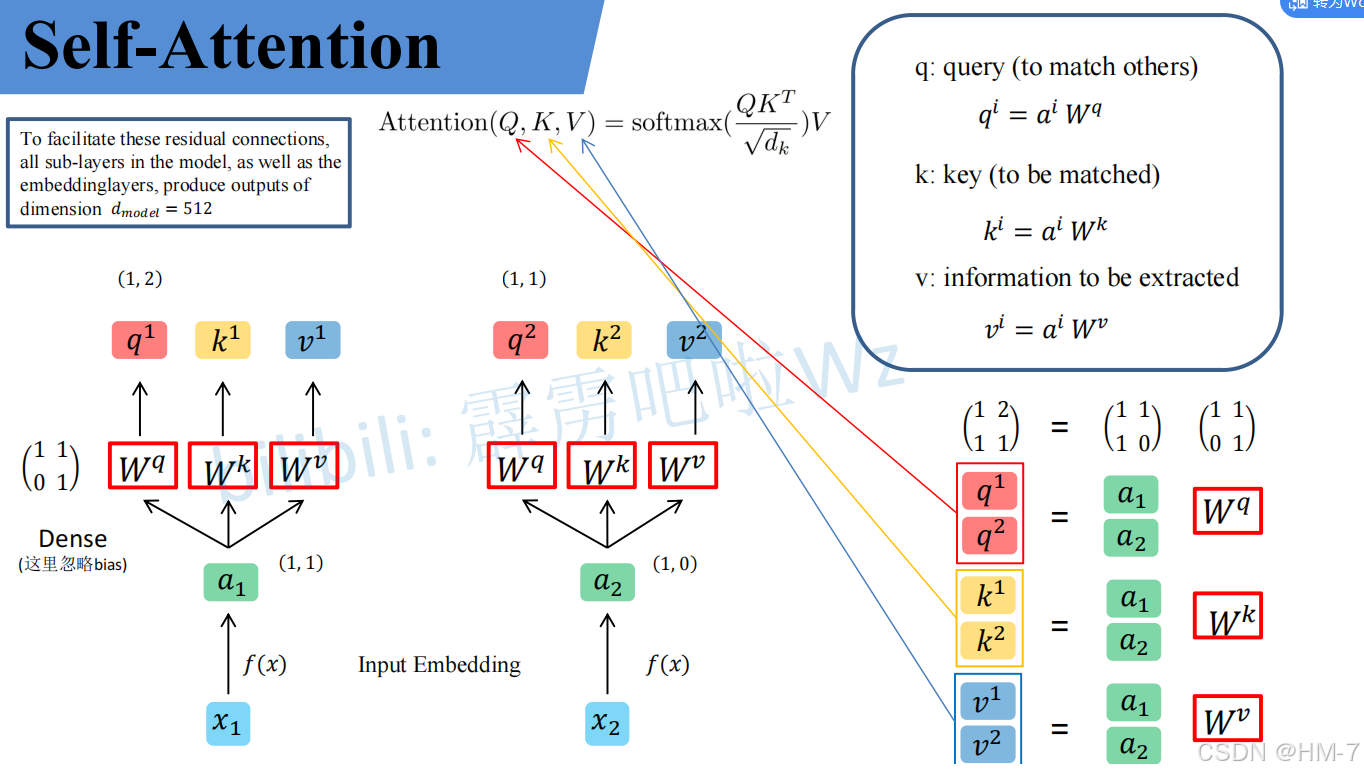
Self-Attention

自注意力机制是广泛用于深度学习的方法，其允许模型在处理输入数据时自动关注不同部分的相关性，从而提高特征提取和表示能力。

具体可分为以下几个步骤：

• 输入嵌入： 输入序列（如词嵌入）被表示为一个矩阵，矩阵的每一行对应一个输入元素（如一个单词的嵌入向量）。

• 生成查询、键和值： 输入嵌入通过三个不同的线性变换生成查询（Query）、键（Key）和值（Value）：

  • 查询（Q）：表示需要关注的部分。
  • 键（K）：表示可被关注的部分。
  • 值（V）：表示对应的输出信息。
    

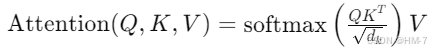
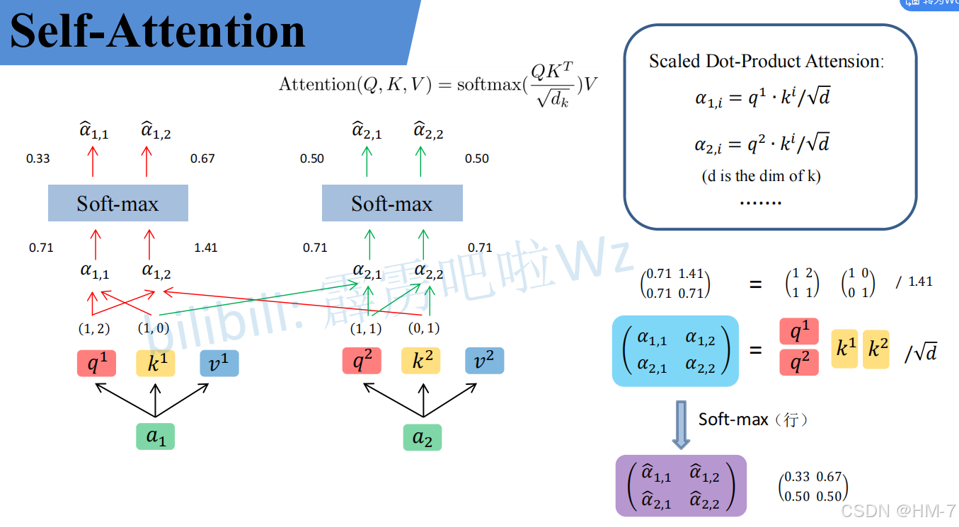
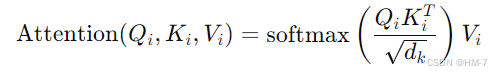
• 计算注意力权重： 通过计算查询与键之间的点积，然后进行缩放和归一化，得到注意力权重：
  
  

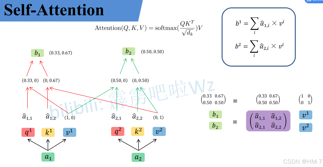
• 加权求和： 使用计算得到的注意力权重对值进行加权求和，得到输出表示。这个表示可以被理解为是对输入序列中不同元素的加权整合。
  

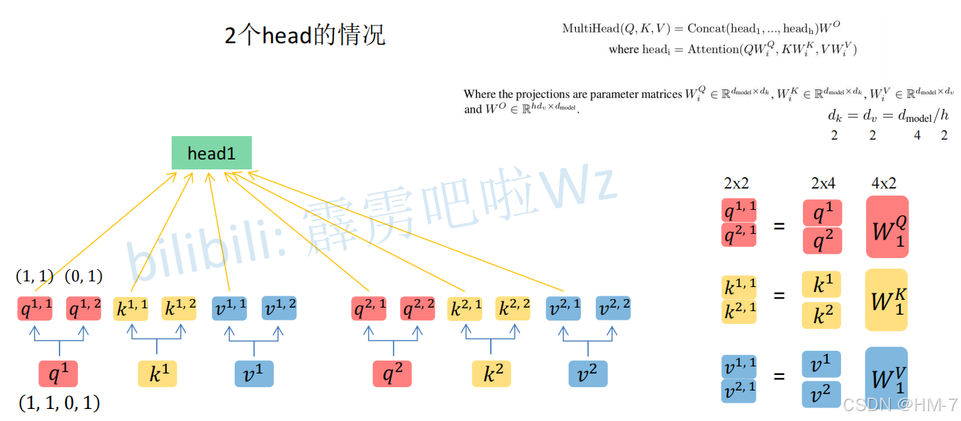
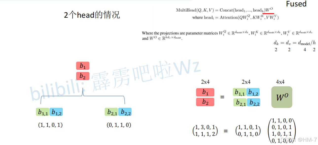
Multi-Head多头注意力

自注意力机制的一种扩展，广泛应用于 Transformer 模型中。它通过并行计算多个自注意力头，允许模型在不同的表示子空间中学习信息，从而增强了模型的表达能力。
（这里有点类似与分组卷积的思想）

工作步骤：

• 输入嵌入： 输入序列（如词嵌入）被表示为一个矩阵，通常是一个三维张量（batch_size, sequence_length, embedding_dim），其实batch_size就是所说的头。

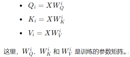
• 线性变换： 对输入的查询、键和值进行线性变换，生成多个头的查询、键和值：

  • 将输入的查询、键和值分别映射到多个不同的子空间中，通常每个子空间的维度为 dk（键的维度）。
  • 对于每个头i有：
    
    

• 计算注意力： 在每个头上，利用注意力机制求注意力权重。
  
  

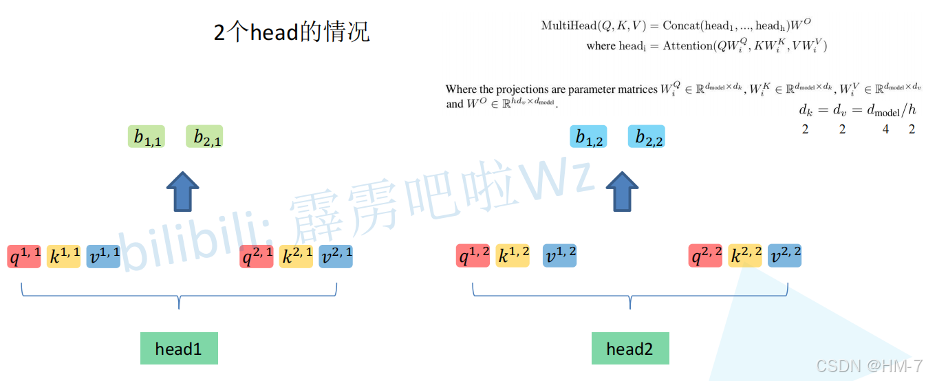
• 合并头的输出： 将所有头的输出拼接起来，并进行线性变换：
  
  

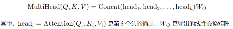
简单实现

自注意力

其实就是矩阵间的点乘和取softmax。
例子来源：https://blog.csdn.net/weixin_44791964/article/details/135423390?fromshare=blogdetail&sharetype=blogdetail&sharerId=135423390&sharerefer=PC&sharesource=qq_51098172&sharefrom=from_link

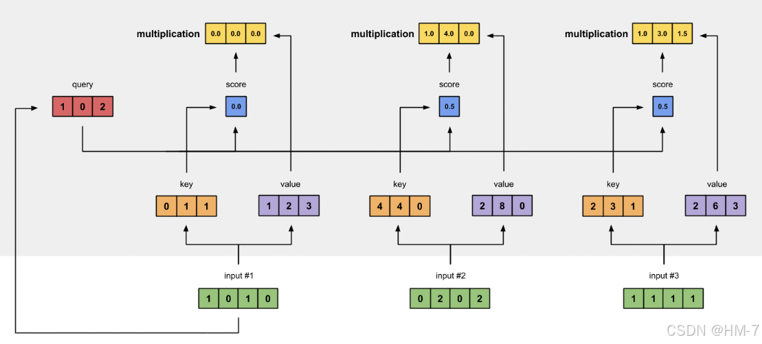
此时我们想求input1的输出：

• 首先利用input1的query去和input1、input2、input3的key相乘，求出的即为score。
• 对求出的三个score求softmax，分别获取到了input1、input2、input3的重要程度。
• 随后将softmax处理后的值与input1、input2、input3的value相乘，再求和。
• 上述步骤后的值即为input1的输出。

多头注意力

假设现在有个特征序列的shape为[3, 768]，也就意味着序列长度为3，每一个单位序列的特征大小为768。

在施加多头的时候，我们直接对[3, 768]的最后一维度进行分割，比如我们想分割成12个头，那么矩阵的shepe就变成了[3, 12, 64]。

然后我们将[3, 12, 64]进行转置，将12放到前面去，获得的特征层为[12, 3, 64]。之后我们忽略这个12，把它和batch维度同等对待，只对3, 64进行处理，其实也就是上面的注意力机制的过程了。

import torch

value_len = 3
num_attention_heads = 12
hidden_size = 768

Query = torch.randn(value_len, hidden_size)
Value = torch.randn(value_len, hidden_size)
Key = torch.randn(value_len, hidden_size)

# 分割出头层
Query = torch.reshape(Query, (value_len, num_attention_heads, hidden_size // num_attention_heads))
Query = torch.transpose(Query, 0, 1)

Value = torch.reshape(Value, (value_len, num_attention_heads, hidden_size // num_attention_heads))
Value = torch.transpose(Value, 0, 1)

Key = torch.reshape(Key, (value_len, num_attention_heads, hidden_size // num_attention_heads))
Key = torch.transpose(Key, 0, 1)

# 求注意力权重
scores = Query @ torch.permute(Key, (0, 2, 1))
scores = torch.softmax(scores, dim=-1)
print(scores.shape)
out = scores @ Value
print(out.shape)
out = torch.permute(out, (1, 0, 2))
print(out.shape)
out = torch.reshape(out, (value_len, hidden_size))
print(out.shape)