


在我设计自主导航系统时:大抵是这样的实现思路:
-
全局路径规划(A*算法获取最短路径)
-
局部运动控制(未来预测模型MPC优化局部运动路径)
-
动态避障与仿真(借用python中的Matplotlib库做可视化仿真
先放出我完整的,很大瑕疵的仿真代码:
虽然从实现思路来讲,仿真是最外层的东西,但实际第一步要考虑的是地图和静动态障碍物设计;
所以有了:(1)创建一个空的零矩阵栅格地图(20*20)和静态障碍物
(2)从我们规划的AStarPlanner类里初始化参数
(3)path是我们得到的全局路径列表
def simulate():
    # 创建地图 (20x20网格,1=障碍物)
    grid = np.zeros((20, 20))
    grid[5:15, 10] = 1  # 设置垂直障碍墙

    # A*路径规划
    planner = AStarPlanner(grid)
    path = planner.plan((1, 1), (18, 18))  # 起点(1,1)到终点(18,18)
随后调用仿真函数
for step in range(100):
    # 更新动态障碍物位置
    obstacles[0][0] += 0.05 if step < 50 else -0.05

    # MPC求解控制量
    u = mpc.solve(x, path, obstacles)

    # 更新AGV状态
    x[0] += u[0] * np.cos(x[2]) * mpc.dt
    x[1] += u[0] * np.sin(x[2]) * mpc.dt
    x[2] += u[1] * mpc.dt
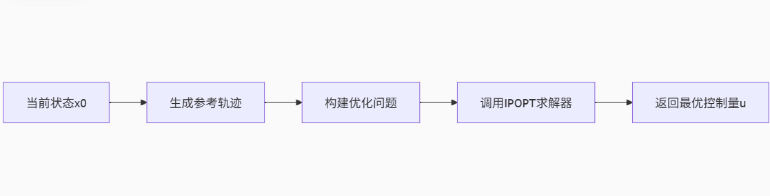
在mpc.solve函数中:处理逻辑如下:
-
参考轨迹生成
-
在全局路径中找到离当前状态最近的点
-
提取未来
N+1个点作为参考轨迹 -
为每个点计算期望朝向角(让AGV看向下一个目标)
-
简单避障处理:如果参考点靠近障碍物,调整朝向角
-
-
优化求解
-
将当前状态
x0和参考轨迹X_ref输入预定义的CasADi模型 -
考虑控制约束(速度
v和角速度ω的范围) -
求解得到未来
N步的最优控制序列
-
其中:CasADi作为一个非线性优化运算处理库也被detect在MPC类中
主要数据传输如:

import numpy as np
import matplotlib.pyplot as plt
import casadi as ca
from scipy.spatial.distance import cdist

# ================== A* 路径规划 ==================
class AStarPlanner:
    def __init__(self, grid):
        self.grid = grid  # 2D地图 (0=空闲, 1=障碍物)
        self.rows, self.cols = grid.shape

    def plan(self, start, goal):
        open_set = {start}
        came_from = {}
        g_score = {start: 0}
        f_score = {start: self._heuristic(start, goal)}

        while open_set:
            current = min(open_set, key=lambda x: f_score[x])
            if current == goal:
                return self._reconstruct_path(came_from, current)

            open_set.remove(current)
            for neighbor in self._get_neighbors(current):
                tentative_g = g_score[current] + 1
                if neighbor not in g_score or tentative_g < g_score[neighbor]:
                    came_from[neighbor] = current
                    g_score[neighbor] = tentative_g
                    f_score[neighbor] = tentative_g + self._heuristic(neighbor, goal)
                    if neighbor not in open_set:
                        open_set.add(neighbor)
        return []  # 无路径

    def _heuristic(self, a, b):
        return np.linalg.norm(np.array(a) - np.array(b))

    def _get_neighbors(self, pos):
        neighbors = []
        for dx, dy in [(-1,0),(1,0),(0,-1),(0,1),(-1,-1),(-1,1),(1,-1),(1,1)]:  # 8-邻域
            x, y = pos[0]+dx, pos[1]+dy
            if 0<=x<self.rows and 0<=y<self.cols and self.grid[x,y]==0:
                neighbors.append((x,y))
        return neighbors

    def _reconstruct_path(self, came_from, current):
        path = [current]
        while current in came_from:
            current = came_from[current]
            path.append(current)
        return path[::-1]

# ================== 改进的MPC控制器 ==================
class MPCController:
    def __init__(self):
        # AGV动力学参数 (状态: x,y,θ; 控制: v,ω)
        self.dt = 0.1
        self.N = 15          # 预测时域
        self.n_states = 3    # 状态维度
        self.n_controls = 2  # 控制维度

        # 权重矩阵 (Q: 状态误差, R: 控制量, F: 终端误差)
        self.Q = np.diag([100, 100, 50])
        self.R = np.diag([50, 5])
        self.F = np.diag([200, 200, 100])

        # 控制约束
        self.v_bounds = (0, 2.0)    # 线速度范围
        self.omega_bounds = (-1.0, 1.0)  # 角速度范围

        # 初始化优化问题
        self._setup_optimizer()
        self.obstacle_weight = 100  # 避障权重

    def _setup_optimizer(self):
        # 定义CasADi优化变量
        self.U = ca.SX.sym('U', self.N * self.n_controls)
        self.X_ref = ca.SX.sym('X_ref', (self.N+1)*self.n_states)
        self.x0 = ca.SX.sym('x0', self.n_states)

        # 构建预测模型
        x_pred = self.x0
        cost = 0
        g = []  # 约束容器

        for i in range(self.N):
            # 当前控制量
            u = self.U[i*self.n_controls : (i+1)*self.n_controls]

            # 动力学模型 (差速驱动模型)
            x_next = ca.vertcat(
                x_pred[0] + u[0]*ca.cos(x_pred[2])*self.dt,
                x_pred[1] + u[0]*ca.sin(x_pred[2])*self.dt,
                x_pred[2] + u[1]*self.dt
            )

            # 代价函数
            x_err = x_pred - self.X_ref[i*self.n_states:(i+1)*self.n_states]
            cost += ca.mtimes([x_err.T, self.Q, x_err])
            cost += ca.mtimes([u.T, self.R, u])

            # 状态传递
            x_pred = x_next

            # 控制量约束
            g.append(u[0])  # v
            g.append(u[1])  # ω

        # 终端代价
        x_err = x_pred - self.X_ref[-self.n_states:]
        cost += ca.mtimes([x_err.T, self.F, x_err])

        # 优化问题设置
        nlp = {'x': self.U, 'f': cost, 'g': ca.vertcat(*g), 'p': ca.vertcat(self.x0, self.X_ref)}
        opts = {'ipopt.print_level': 0, 'print_time': 0}
        self.solver = ca.nlpsol('solver', 'ipopt', nlp, opts)

    def solve(self, x0, path_ref, obstacles=None):
        # 生成参考轨迹 (前瞻点)
        ref_traj = self._generate_reference(x0, path_ref, obstacles)
        X_ref = ref_traj.flatten()

        # 优化参数
        p = np.concatenate([x0, X_ref])

        # 约束上下界
        lbg = [self.v_bounds[0], self.omega_bounds[0]] * self.N
        ubg = [self.v_bounds[1], self.omega_bounds[1]] * self.N

        # 求解MPC问题
        res = self.solver(p=p, lbg=lbg, ubg=ubg)
        u_opt = res['x'].full().flatten()

        return u_opt[:self.n_controls]  # 返回第一步控制

    def _generate_reference(self, x0, path_ref, obstacles):
        # 从全局路径中找到最近点
        if len(path_ref) == 0:
            return np.tile(x0, (self.N+1, 1))

        distances = cdist([x0[:2]], path_ref)
        closest_idx = np.argmin(distances)

        # 提取前瞻点
        ref_traj = []
        for i in range(self.N+1):
            idx = min(closest_idx + i, len(path_ref)-1)
            target = path_ref[idx]

            # 计算期望朝向角
            if i < self.N and idx+1 < len(path_ref):
                next_target = path_ref[idx+1]
                theta_ref = np.arctan2(next_target[1]-target[1], next_target[0]-target[0])
            else:
                theta_ref = x0[2]  # 保持当前朝向

            # 避障惩罚 (简单基于障碍物的距离进行惩罚)
            for obs in obstacles:
                dist = np.linalg.norm(np.array([target[0], target[1]]) - np.array([obs[0], obs[1]]))
                if dist < obs[2]:
                    # 增加避障惩罚项
                    theta_ref += np.pi / 4  # 示例:避障方向调整

            ref_traj.append([target[0], target[1], theta_ref])

        return np.array(ref_traj)

# ================== 主仿真循环 ==================
def simulate():
    # 创建地图 (1=障碍物)
    grid = np.zeros((20, 20))
    grid[5:15, 10] = 1  # 静态障碍物 (墙)

    # A* 规划全局路径
    planner = AStarPlanner(grid)
    path = planner.plan((1, 1), (18, 18))
    if not path:
        print("A* 无法找到路径!")
        return

    # 初始化MPC控制器
    mpc = MPCController()

    # 动态障碍物 [x, y, 半径]
    obstacles = [[15, 15, 1.5]]

    # AGV初始状态 [x, y, theta]
    x = np.array([1.0, 1.0, 0.0])

    # 存储轨迹用于可视化
    trajectory = [x.copy()]

    # 可视化初始化
    plt.figure(figsize=(10, 8))
    for step in range(100):
        # 更新动态障碍物 (示例:周期性移动)
        obstacles[0][0] += 0.05 if step < 50 else -0.05

        # MPC控制
        u = mpc.solve(x, path, obstacles)

        # 状态更新 (前向欧拉积分)
        x[0] += u[0] * np.cos(x[2]) * mpc.dt
        x[1] += u[0] * np.sin(x[2]) * mpc.dt
        x[2] += u[1] * mpc.dt
        trajectory.append(x.copy())

        # 可视化
        plt.clf()
        plt.imshow(grid.T, origin='lower', cmap='Greys', alpha=0.3)

        # 绘制路径和轨迹
        path_array = np.array(path)
        plt.plot(path_array[:,0], path_array[:,1], 'g--', label='全局路径')
        traj_array = np.array(trajectory)
        plt.plot(traj_array[:,0], traj_array[:,1], 'b-', label='AGV轨迹')
        plt.plot(x[0], x[1], 'bo', markersize=8, label='AGV当前位置')

        # 绘制障碍物
        for obs in obstacles:
            circle = plt.Circle((obs[0], obs[1]), obs[2], color='r', alpha=0.3)
            plt.gca().add_patch(circle)

        plt.legend()
        plt.xlim(0, 20)
        plt.ylim(0, 20)
        plt.title(f'Step: {step}, 控制量: v={u[0]:.2f}, ω={u[1]:.2f}')
        plt.pause(0.05)

        # 检查是否到达目标
        if np.linalg.norm(x[:2] - path[-1]) < 0.5:
            print("到达目标!")
            break

    plt.show()

if __name__ == "__main__":
    simulate()
到此,一个工程文件的仿真初步架构结束;
接下来我们分析仿真问题
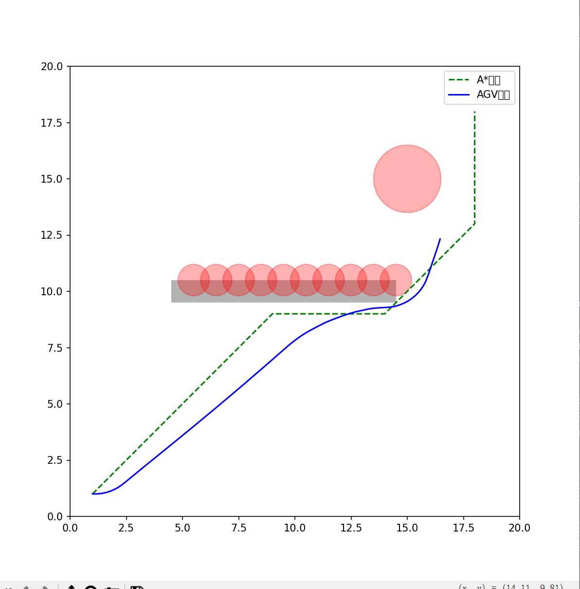
仿真结果如图:
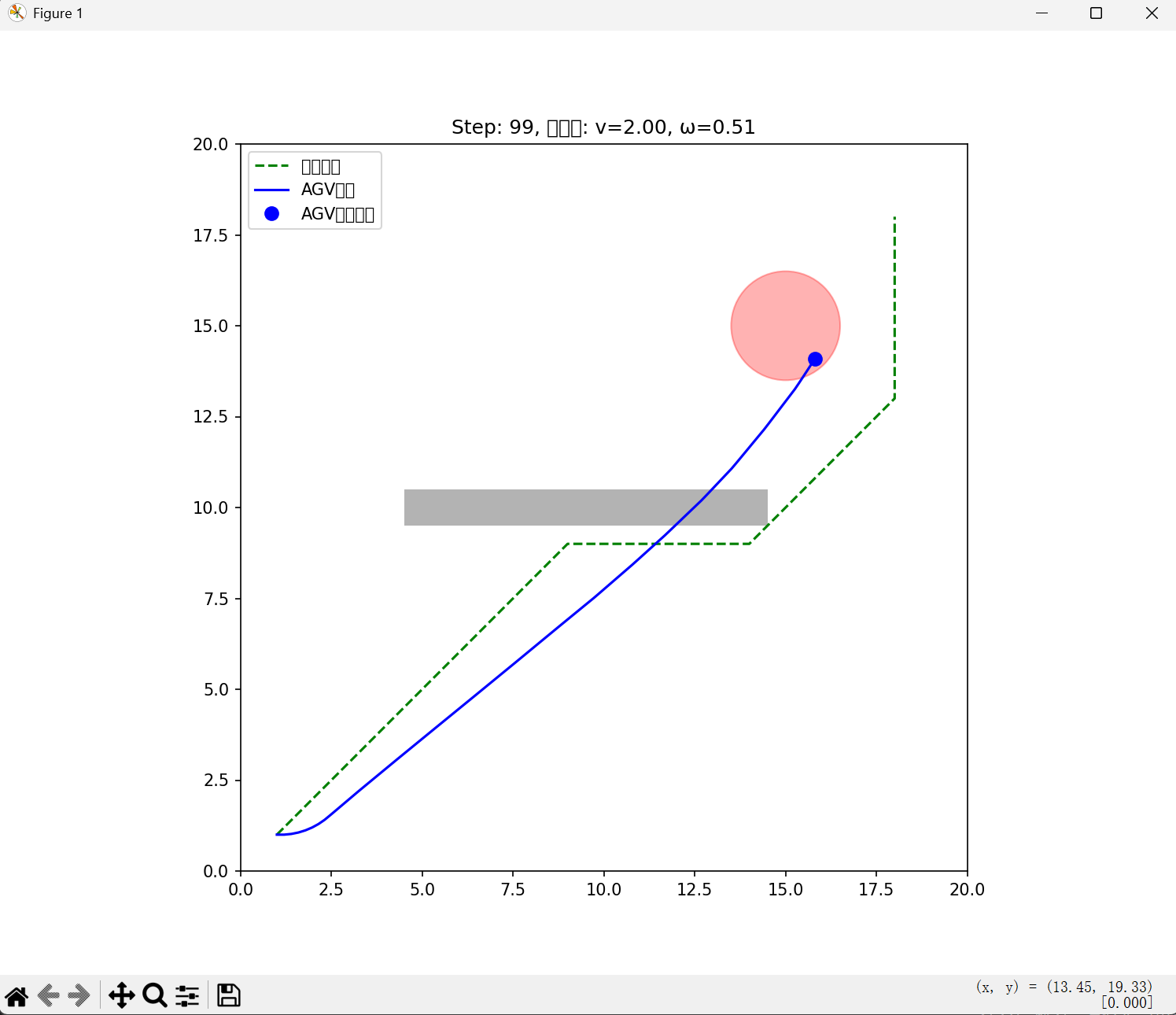
显然:在Actual-path中,无视掉了障碍物
这是一个综合性的问题:它来自
1 主优化器没有接入正确格式的path数据/没有写入
2 MPC和A*对path的权重影响不同:我们可以清楚看到,在全局最优路径正确反映出来的前提下:由于MPC的局部处理高权重影响,它忽略了全局路径和障碍物惩罚
3 障碍物惩罚权重仍然不够:在程序中
 self.obstacle_weight = 100  # 避障权
 # 避障惩罚
 for obs in obstacles:
       dist = np.linalg.norm(np.array([target[0], target[1]]) - np.array([obs[0], obs[1]]))
          if dist < obs[2]:
                    # 增加避障惩罚项
                    theta_ref += np.pi / 4  # 示例:避障方向调整

       ref_traj.append([target[0], target[1], theta_ref])
这个障碍惩罚显然有些轻薄,我们要更换更严厉的惩罚权重:比如:
obs_weight = k(a+ 1/dist[0.1])(分母常数项)
或者指数爆炸型:
cost += self.obstacle_weight * ca.fmax(h, 0)**2
优化结果:
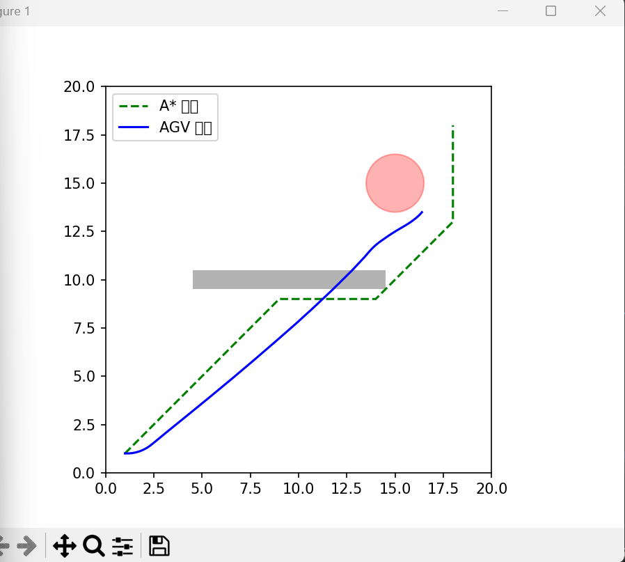
到这里为止,可以发现最大的问题:
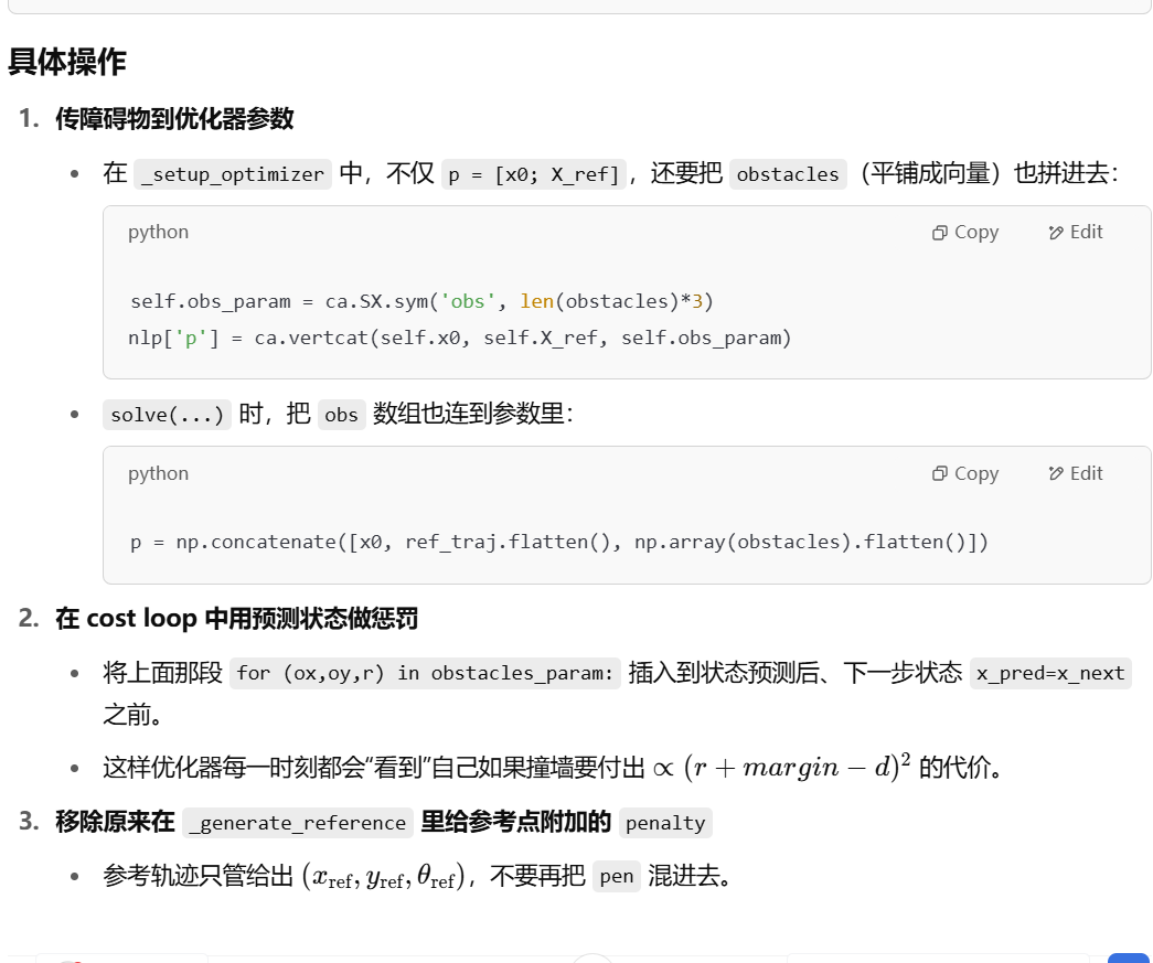
障碍物和处理后的路径显然没有写入主优化器
(以下建议来自chatgpt-4o)
随即附上更新后的完整code:
import numpy as np
import matplotlib.pyplot as plt
import casadi as ca
from scipy.spatial.distance import cdist

# ================== A* 路径规划 ==================
class AStarPlanner:
    def __init__(self, grid):
        self.grid = grid
        self.rows, self.cols = grid.shape

    def plan(self, start, goal):
        open_set = {start}
        came_from = {}
        g_score = {start: 0}
        f_score = {start: self._heuristic(start, goal)}
        while open_set:
            current = min(open_set, key=lambda x: f_score[x])
            if current == goal:
                return self._reconstruct_path(came_from, current)
            open_set.remove(current)
            for nbr in self._get_neighbors(current):
                tentative = g_score[current] + 1
                if nbr not in g_score or tentative < g_score[nbr]:
                    came_from[nbr] = current
                    g_score[nbr] = tentative
                    f_score[nbr] = tentative + self._heuristic(nbr, goal)
                    open_set.add(nbr)
        return []

    def _heuristic(self, a, b):
        return np.linalg.norm(np.array(a) - np.array(b))

    def _get_neighbors(self, pos):
        nbrs = []
        for dx, dy in [(-1,0),(1,0),(0,-1),(0,1),(-1,-1),(-1,1),(1,-1),(1,1)]:
            x, y = pos[0]+dx, pos[1]+dy
            if 0<=x<self.rows and 0<=y<self.cols and self.grid[x,y]==0:
                nbrs.append((x,y))
        return nbrs

    def _reconstruct_path(self, came_from, curr):
        path = [curr]
        while curr in came_from:
            curr = came_from[curr]
            path.append(curr)
        return path[::-1]

# ================== 改进的 MPC 控制器 ==================
class MPCController:
    def __init__(self, obstacles):
        # ----- 基本参数 -----
        self.dt = 0.1
        self.N = 15
        self.n_states = 3   # x, y, θ
        self.n_controls = 2 # v, ω

        # ----- 权重 -----
        self.Q = np.diag([50, 50, 20])
        self.R = np.diag([50, 5])
        self.F = np.diag([200, 200, 100])
        self.obstacle_weight = 1e4   # W_obs,大幅增大“撞墙成本”


        # 每个元素 [ox, oy, radius]
        self.obstacles = np.array(obstacles)
        self.n_obs = self.obstacles.shape[0]


        self.v_bounds     = (0.0, 2.0)
        self.omega_bounds = (-1.0, 1.0)

        # 构建 CasADi 优化器
        self._setup_optimizer()

    def _setup_optimizer(self):
        # 决策变量 U
        self.U = ca.SX.sym('U', self.N*self.n_controls)
        # 参考轨迹 (x_ref, y_ref, θ_ref), 展平
        self.X_ref = ca.SX.sym('X_ref', (self.N+1)*3)
        # 初始状态
        self.x0    = ca.SX.sym('x0', 3)
        # 障碍物参数: [ox1,oy1,r1, ox2,oy2,r2, ...]
        self.obs_p = ca.SX.sym('obs_p', 3*self.n_obs)

        cost = 0
        g_list = []
        x_pred = self.x0

        # 逐步构造 cost & 约束
        for i in range(self.N):
            # current control
            u = self.U[2*i:2*i+2]
            # dynamics
            x_next = ca.vertcat(
                x_pred[0] + u[0]*ca.cos(x_pred[2])*self.dt,
                x_pred[1] + u[0]*ca.sin(x_pred[2])*self.dt,
                x_pred[2] + u[1]*self.dt
            )
            # 路径跟踪误差
            idx = 3*i
            x_err = x_pred - self.X_ref[idx:idx+3]
            cost += ca.mtimes([x_err.T, self.Q, x_err])
            # 控制量平滑
            cost += ca.mtimes([u.T, self.R, u])
            # ----- 直接对预测状态做障碍物二次惩罚 -----
            margin = 0.5
            for j in range(self.n_obs):
                ox = self.obs_p[3*j]
                oy = self.obs_p[3*j+1]
                r  = self.obs_p[3*j+2]
                dx = x_pred[0] - ox
                dy = x_pred[1] - oy
                dist_pred = ca.sqrt(dx*dx + dy*dy)
                h = (r + margin) - dist_pred

                cost += self.obstacle_weight * ca.fmax(h, 0)**2


            x_pred = x_next
            g_list += [u[0], u[1]]

        # 终端误差
        idx_end = 3*self.N
        x_err_end = x_pred - self.X_ref[idx_end:idx_end+3]
        cost += ca.mtimes([x_err_end.T, self.F, x_err_end])

        # NLP 设定
        g_cat = ca.vertcat(*g_list)
        p = ca.vertcat(self.x0, self.X_ref, self.obs_p)
        nlp = {'x': self.U, 'f': cost, 'g': g_cat, 'p': p}
        opts = {'ipopt.print_level':0, 'print_time':0}
        self.solver = ca.nlpsol('solver', 'ipopt', nlp, opts)

    def solve(self, x0, path_ref):
        ref = self._generate_reference(x0, path_ref)
        obs_arr = np.array(self.obstacles)       # ← 转成 ndarray
        p_vec = np.concatenate([
        x0,
        ref.flatten(),
        obs_arr.flatten()
    ])


        lbg = [self.v_bounds[0], self.omega_bounds[0]]*self.N
        ubg = [self.v_bounds[1], self.omega_bounds[1]]*self.N

        sol = self.solver(p=p_vec, lbg=lbg, ubg=ubg)
        u_opt = sol['x'].full().flatten()
        return u_opt[:2]

    def _generate_reference(self, x0, path_ref):

        if not path_ref:

            return np.tile(x0, (self.N+1,1))
        dists = cdist([x0[:2]], path_ref)
        idx0 = np.argmin(dists)

        traj = []
        for i in range(self.N+1):
            idx = min(idx0+i, len(path_ref)-1)
            tx, ty = path_ref[idx]
            # 计算朝向
            if idx < len(path_ref)-1:
                nx, ny = path_ref[idx+1]
                th = np.arctan2(ny-ty, nx-tx)
            else:
                th = x0[2]
            traj.append([tx, ty, th])
        return np.array(traj)

# ================== 主仿真循环 ==================
def simulate():

    grid = np.zeros((20,20))
    grid[5:15,10] = 1


    planner = AStarPlanner(grid)
    path = planner.plan((1,1), (18,18))
    if not path:
        print("A* 无解")
        return


    static_cells = np.argwhere(grid==1)
    static_obs = []
    for row, col in static_cells:
    # 直接把 row→y, col→x
        static_obs.append([ row+0.5,col+0.5, 0.7])


    dynamic_obs = [[15, 15, 1.5]]


    obstacles = static_obs + dynamic_obs
    mpc = MPCController(obstacles)


    x = np.array([1.0,1.0,0.0])
    traj = [x.copy()]

    plt.figure(figsize=(8,8))
    for step in range(100):

        dynamic_obs[0][0] += 0.05 if step<50 else -0.05

        mpc.obstacles = static_obs + dynamic_obs

        # 求 MPC 控制
        u = mpc.solve(x, path)
        # 状态更新
        x = x + np.array([
            u[0]*np.cos(x[2])*mpc.dt,
            u[0]*np.sin(x[2])*mpc.dt,
            u[1]*mpc.dt
        ])
        traj.append(x.copy())


        plt.clf()
        plt.imshow(grid.T, origin='lower', cmap='Greys', alpha=0.3)
        path_arr = np.array(path)
        plt.plot(path_arr[:,0], path_arr[:,1], 'g--', label='A*路径')
        tr = np.array(traj)
        plt.plot(tr[:,0], tr[:,1], 'b-', label='AGV轨迹')

        for ox, oy, r in mpc.obstacles:
            plt.gca().add_patch(plt.Circle((ox,oy), r, color='r', alpha=0.3))
        plt.legend(); plt.xlim(0,20); plt.ylim(0,20)
        plt.pause(0.05)

        if np.linalg.norm(x[:2]-path[-1])<0.5:
            print("到达目标")
            break

    plt.show()


if __name__ == "__main__":
    simulate()


# ================== 主仿真循环 ==================
def simulate():
    # 地图
    grid = np.zeros((20,20))
    grid[5:15,10] = 1

    # A*
    planner = AStarPlanner(grid)
    path = planner.plan((1,1),(18,18))
    if not path:
        print("A* 无解"); return

    # MPC
    mpc = MPCController()
    obstacles = [[15,15,1.5]]

    x = np.array([1.0,1.0,0.0])
    traj = [x.copy()]

    plt.figure(figsize=(8,8))
    for step in range(100):
        # 动态障碍
        obstacles[0][0] += 0.05 if step<50 else -0.05
        # 求 MPC 控制
        u = mpc.solve(x, path, obstacles)
        # 前向欧拉
        x = x + np.array([
            u[0]*np.cos(x[2])*mpc.dt,
            u[0]*np.sin(x[2])*mpc.dt,
            u[1]*mpc.dt
        ])
        traj.append(x.copy())

        plt.clf()
        plt.imshow(grid.T,origin='lower',cmap='Greys',alpha=0.3)
        path_arr = np.array(path)
        plt.plot(path_arr[:,0], path_arr[:,1],'g--',label='A*路径')
        ta = np.array(traj)
        plt.plot(ta[:,0], ta[:,1],'b-',label='AGV轨迹')
        for ox,oy,r in obstacles:
            circle = plt.Circle((ox,oy),r,color='r',alpha=0.3)
            plt.gca().add_patch(circle)
        plt.legend(); plt.xlim(0,20); plt.ylim(0,20)
        plt.pause(0.05)
        if np.linalg.norm(x[:2]-path[-1])<0.5:
            print("到达目标"); break
    plt.show()

if __name__ == "__main__":
    simulate()
仿真结果如图:
至此:一个可以用的混合A*+MPC综合控制避障仿真结束;
下一篇我会专门就中间迭代版本差异做分享学习,并尝试混合A*和CBF算法加强介入


 4931
4931

 被折叠的 条评论
为什么被折叠?
被折叠的 条评论
为什么被折叠?
 到【灌水乐园】发言


