深度学习训练营之J5周DenseNet+SE-Net实战

无你想你

已于 2023-06-02 22:37:15 修改

阅读量518

点赞数 1

分类专栏：深度学习文章标签：深度学习人工智能计算机视觉

于 2023-06-02 21:35:57 首次发布

本文链接：https://blog.csdn.net/qq_62904883/article/details/131014187

版权

深度学习专栏收录该内容

27 篇文章 1 订阅

订阅专栏

深度学习训练营之J5周DenseNet+SE-Net实战

原文链接
方法介绍
SE模块应用分析
SE模块的效果对比
SE模块代码实现
SE模块在DenseNet当中的应用
参考内容

原文链接

📌第J5周：DenseNet+SE-Net实战📌

🍨 本文为🔗365天深度学习训练营中的学习记录博客
🍖 原作者：K同学啊|接辅导、项目定制

语言：Python3、Pytorch
📌本周任务：📌

1. 在DenseNet系列算法中插入SE-Net通道注意力机制，并完成猴痘病识别
1. 改进思路是否可以迁移到其他地方呢
3.测试集accuracy达到89%（拔高，可选）

🔊注：从前几周开始训练营的难度逐渐提升，具体体现在不再直接提供源代码。任务中会给大家提供一些算法改进的思路、方向，希望大家这一块可以积极探索。（这个探索的过程很重要，也将学到更多）
个人感悟:本周由于临近期末考试,本周三进行数学专业课程的考试,然后还加上重感冒,所以这一次的深度学习训练营所准备的时间还是不是很充足,而且在DenseNet的实际应用上可以明显感觉到自身能力的不足,所以本次在代码的实现过程当中还是有点不熟练,所以本次主要以方法介绍为主,给大家带来的不便感到十分抱歉
论文链接:Squeeze-and-Excitation Networks

方法介绍

SE-Net作为ImageNet 2017 的冠军模型,其优点如下:

复杂度低
计算量小

其具体策略为：通过学习的方式来自动获取到每个特征通道的重要程度，然后依照这个重要程度去提升有用的特征并抑制对当前任务用处不大的特征，这又叫做“特征重标定”策略。具体的SE模块如下图所示
请添加图片描述
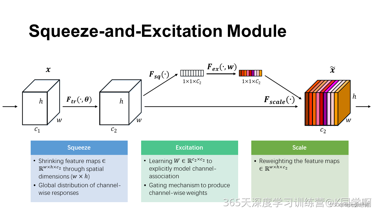
给定一个输入 $x$ ,其特征通道数为 $c_1$ ,经过一系列卷积等一般变换 $F_{tr}$ ,后得到一个特征通道数为 $c_2$ 的特征。与传统的卷积神经网络不同，我们需要通过下面三个操作来重新标定前面得到的特征。

1.首先是Squeeze操作，我们顺着空间维度来进行特征压缩，将一个通道数和输入的特征通道数相等，例如可以将将形状为(1, 32, 32, 10)的feature map压缩成(1, 1, 1, 10)。此操作通常采用global average pooling来实现。
2.得到了全局描述特征后，我们进行Excitation操作来抓取特征通道之间的关系，它是一个类似于循环神经网络中门的机制：
$s=F_{e x}(z, W)=\sigma(g(z, W))=\sigma\left(W_{2} \operatorname{Re} L U\left(W_{1} z\right)\right)$

这里采用包含两个全连接层的bottleneck结构，即中间小两头大的结构：其中第一个全链接层起到即降维的作用，并通过ReLU激活，第二个全链接层用来将其恢复至原始的维度。进行Excitation操作的最终目的是为每个特征通道生成权重，即学习到的各个通道的激活值（sigmoid激活，值在0~1之间）。
最后一个是Scale的操作，我们将Excitation的输出的权重看作是经过特征选择后的每个特征通道的重要性，然后通过乘法逐通道加权到先前的特征上，完成在通道维度上的对原始特征的重标定，从而提高了每一个通道在模型上的特征更有辨别能力,这类似于attention机制。

SE模块应用分析

请添加图片描述
SE模块非常灵活,表现在其可以直接应用在现有的网络结果中,以Inception和ResNet为例,可以直接在这两个模块后面添加SE模块

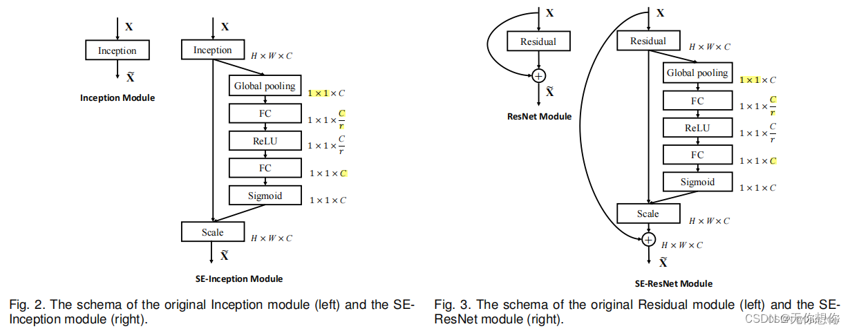
方框旁边的维度信息代表该层的输出, $r$ 表示Excitation(激发)操作当中的降维系数

SE模块的效果对比

在ImageNet上的效果
请添加图片描述
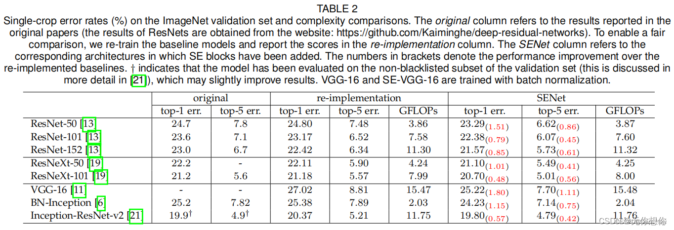
从上表可以看出，SE-ResNets在各种深度上都远远超过了其对应的没有SE的结构版本的精度,这表示无论网络的深度以及大小，SE模块都能够给网络带来性能上的增益。值得一提的是，SE-ResNet-50可以达到和ResNet-101一样的精度；更甚，SE-ResNet-101远远地超过了更深的ResNet-152

SE模块代码实现

tensorflow

from tensorflow import keras
from keras import layers
from layers import Model, Input, Reshape, Activation, BatchNormalization, GlobalAveragePooling2D, Dense

class SqueezeExcitationLayer(Model):
    def __init__(self, filter_sq):
        # filter_sq是Excitation中第一个卷积过程中卷积核的个数
        super.__init__()
        self.avgpool = GlobalAveragePooling2D()
        self.dense = Dense(filter_sq)
        self.relu = Activation('relu')
        self.sigmoid = Activation('sigmoid')
    
    def call(self, inputs):
        x = self.avgpool(inputs)
        x = self.dense(x)
        x = self.relu(x)
        x = Dense(inputs.shape[-1])(x)
        x = self.sigmoid(x)
        x = Reshape((1,1,inputs.shape[-1]))(x)
        
        scale = inputs * x
        return scale

SE = SqueezeExcitationLayer(16)

SE模块在DenseNet当中的应用

tensorflow

''' Basic unit of DenseBlock (using bottleneck layer) '''
def DenseLayer(x, bn_size, growth_rate, drop_rate, name=None):
    f = BatchNormalization(name=name+'_1_bn')(x)
    f = Activation('relu', name=name+'_1_relu')(f)
    f = Conv2D(bn_size*growth_rate, 1, strides=1, use_bias=False, name=name+'_1_conv')(f)
    
    f = BatchNormalization(name=name+'_2_bn')(f)
    f = Activation('relu', name=name+'_2_relu')(f)
    f = Conv2D(growth_rate, 3, strides=1, padding=1, use_bias=False, name=name+'_2_conv')(f)
    
    if drop_rate>0:
        f = Dropout(drop_rate)(f)
    
    x = layers.Concatenate(axis=-1)([x, f])
    return x


''' DenseBlock '''
def DenseBlock(x, num_layers, bn_size, growth_rate, drop_rate, name=None):
    for i in range(num_layers):
        x = DenseLayer(x, bn_size, growth_rate, drop_rate, name=name+'_denselayer'+str(i+1))
    return x


''' Transition layer between two adjacent DenseBlock '''
def Transition(x, out_channel):
    x = BatchNormalization(name=name+'_bn')(x)
    x = Activation('relu', name=name+'_relu')(x)
    x = Conv2D(out_channel, 1, strides=1, use_bias=False, name=name+'_conv')(x)
    x = AveragePooling2D(2, 2, name='pool')(x)
    return x


''' DenseNet-BC model '''
def DenseNet(input_tensor=None,  # 可选的keras张量，用作模型的图像输入
             input_shape=None,
             init_channel=64,
             growth_rate=32,
             block_config=(6,12,24,16),
             bn_size=4,
             compression_rate=0.5,
             drop_rate=0,
             classes=1000):  # 用于分类图像的可选类数
    img_input = Input(shape=input_shape)
    # first Conv2d
    x = ZeroPadding2D(padding=((3, 3), (3, 3)), name='conv1_pad')(img_input)
    x = Conv2D(64, 7, strides=2, use_bias=False, name='conv1_conv')(x)
    x = BatchNormalization(name='conv1_bn')(x)
    x = Activation('relu', name='conv1_relu')(x)
    x = MaxPooling2D(3, strides=2, padding=1, name='conv1_pool')(x)
    # DenseBlock
    num_features = init_channel
    for i, num_layers in enumerate(block_config):
        x = DenseBlock(x, num_layers, bn_size, growth_rate, drop_rate, name='denseblock'+str(i+1))
        num_features += num_layers*growth_rate
        if i!=len(block_config)-1:
            x = Transition(x, int(num_features*compression_rate))
            num_features = int(num_features*compression_rate)
    # 加SE注意力机制
    x = SqueezeExcitationLayer(16)(x)
    # final bn+ReLU
    x = BatchNormalization(name='final_bn')(x)
    x = Activation('relu', name='final_relu')(x)
    x = GlobalAveragePooling2D(name='final_pool')(x)
    x = Dense(classes, activation='softmax', name='predictions')(x)
    
    model = Model(img_input, x, name='DenseNet')
    return model


''' DenseNet121 '''
def densenet121(n_classes=1000, **kwargs):
    model = DenseNet(init_channel=64, growth_rate=32, block_config=(6,12,24,16),
                     classes=n_classes, **kwargs)
    return model


''' DenseNet169 '''
def DenseNet169(n_classes=1000, **kwargs):
    model = DenseNet(init_channel=64, growth_rate=32, block_config=(6,12,32,32),
                     classes=n_classes, **kwargs)
    return model


''' DenseNet201 '''
def DenseNet201(n_classes=1000, **kwargs):
    model = DenseNet(init_channel=64, growth_rate=32, block_config=(6,12,48,32),
                     classes=n_classes, **kwargs)
    return model