Conv1d 一维卷积图解

新缸中之脑

于 2024-07-23 12:46:17 发布

阅读量958

点赞数 10

文章标签：深度学习

本文链接：https://blog.csdn.net/shebao3333/article/details/140632930

版权

在深度学习中，卷积层是许多深度神经网络的主要构建块。该设计的灵感来自视觉皮层，其中单个神经元对视野的受限区域（称为感受野）做出反应。这些区域的集合重叠以覆盖整个可见区域。

虽然卷积层最初应用于计算机视觉，但其平移不变特性使卷积层可以应用于自然语言处理、时间序列、推荐系统和信号处理。

理解卷积的最简单方法是将其视为应用于矩阵的滑动窗口函数。本文将了解一维卷积的工作原理并探讨每个参数的影响。

NSDT工具推荐： Three.js AI纹理开发包 - YOLO合成数据生成器 - GLTF/GLB在线编辑 - 3D模型格式在线转换 - 可编程3D场景编辑器 - REVIT导出3D模型插件 - 3D模型语义搜索引擎 - Three.js虚拟轴心开发包 - 3D模型在线减面 - STL模型在线切割

1、卷积是如何工作的？（核大小 = 1）

卷积（convolution）是一种线性运算，涉及将权重与输入相乘并产生输出。乘法是在输入数据数组和权重数组 — 称为核（kernel）—之间执行的。在输入和核之间应用的运算是元素点积的总和。每个运算的结果都是一个值。

让我们从最简单的示例开始，当你拥有 1D 数据时使用 1D 卷积。对 1D 数组应用卷积会将核中的值与输入向量中的每个值相乘。

假设核中的值（也称为“权重”）为“2”，我们将输入向量中的每个元素逐个乘以 2，直到输入向量的末尾，并得到输出向量。输出向量的大小与输入的大小相同。

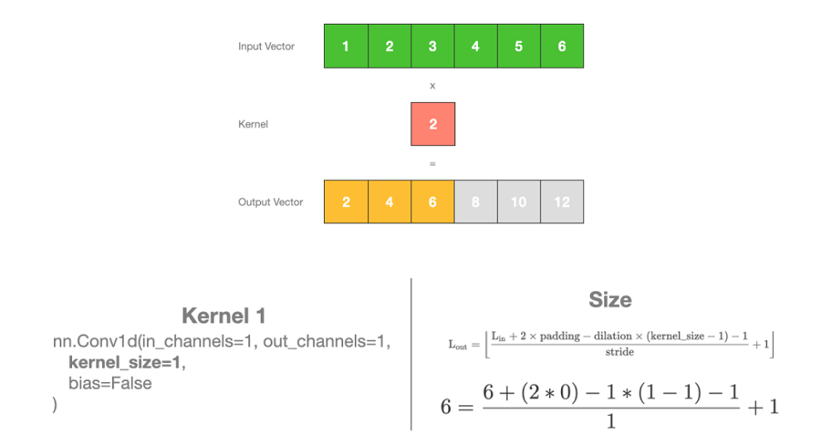
首先，我们将 1 乘以权重 2，得到第一个元素的值为“2”。然后我们将核移动 1 步，将 2 乘以权重 2，得到“4”。我们重复此操作直到最后一个元素 6，然后将 6 乘以权重，得到“12”。此过程生成输出向量。

class TestConv1d(nn.Module):
    def __init__(self):
        super(TestConv1d, self).__init__()
        self.conv = nn.Conv1d(in_channels=1, out_channels=1, kernel_size=1, bias=False)
        self.init_weights()

    def forward(self, x):
        return self.conv(x)
    
    def init_weights(self):
        self.conv.weight[0,0,0] = 2.


in_x = torch.tensor([[[1,2,3,4,5,6]]]).float()
print("in_x.shape", in_x.shape)
print(in_x)

net = TestConv1d()
out_y = net(in_x)

print("out_y.shape", out_y.shape)
print(out_y)

输入如下：

in_x.shape torch.Size([1, 1, 6])  
tensor([[[1., 2., 3., 4., 5., 6.]]])  
out_y.shape torch.Size([1, 1, 6])  
tensor([[[ 2.,  4.,  6.,  8., 10., 12.]]], grad_fn=<SqueezeBackward1>)

2、核大小的影响（核大小 = 2）

不同大小的核将检测输入中不同大小的特征，进而产生不同大小的特征图（feature map）。让我们看另一个示例，其中核大小为 1x2，权重为“2”。像以前一样，我们将核滑过输入向量的每个元素。我们通过将每个元素乘以核并将乘积相加来执行卷积以获得最终输出值。我们一个接一个地重复这种乘法和加法，直到输入向量的末尾，并产生输出向量。

首先，我们将 1 乘以 2 得到“2”，将 2 乘以 2 得到“2”。然后我们将 2 和 4 这两个数字相加，得到“6”——这是输出向量中的第一个元素。我们重复相同的过程，直到输入向量结束，并生成输出向量。

class TestConv1d(nn.Module):
    def __init__(self):
        super(TestConv1d, self).__init__()
        self.conv = nn.Conv1d(in_channels=1, out_channels=1, kernel_size=2, bias=False)
        self.init_weights()

    def forward(self, x):
        return self.conv(x)
    
    def init_weights(self):
        self.conv.weight[0,0,0] = 2.
        self.conv.weight[0,0,1] = 2.


in_x = torch.tensor([[[1,2,3,4,5,6]]]).float()
print("in_x.shape", in_x.shape)
print(in_x)

net = TestConv1d()
out_y = net(in_x)

print("out_y.shape", out_y.shape)
print(out_y)

输出如下：

in_x.shape torch.Size([1, 1, 6])  
tensor([[[1., 2., 3., 4., 5., 6.]]])  
out_y.shape torch.Size([1, 1, 5])  
tensor([[[ 6., 10., 14., 18., 22.]]], grad_fn=<SqueezeBackward1>)

3、计算输出向量的形状

你可能已经注意到，输出向量比以前略小。这是因为我们将核的大小从 1x1 增加到了 1x2。查看 PyTorch 文档，我们可以使用以下方法计算输出向量的长度：

如果我们将大小为 1x2 的核应用于大小为 1x6 的输入向量，我们可以相应地替换值并得到 1x5 的输出长度：

如果你正在构建神经网络架构，则计算输出特征的大小至关重要。

4、核大小通常为奇数（核大小 = 3）

在上例中，核大小为 2 的情况并不常见，因此我们再举一个例子，其中核大小为 3，其权重为“2”。像之前一样，我们通过将每个元素乘以核并将乘积相加来执行卷积。我们重复此过程，直到输入向量结束，从而产生输出向量。

同样，输出向量小于输入向量。在 1x6 输入向量上应用 1x3 核将产生大小为 1x4 的特征向量。

在图像处理中，通常使用 3×3、5×5 大小的核。有时我们可能会对较大的输入图像使用大小为 7×7 的核。

class TestConv1d(nn.Module):
    def __init__(self):
        super(TestConv1d, self).__init__()
        self.conv = nn.Conv1d(in_channels=1, out_channels=1, kernel_size=3, bias=False)
        self.init_weights()

    def forward(self, x):
        return self.conv(x)
    
    def init_weights(self):
        new_weights = torch.ones(self.conv.weight.shape) * 2.
        self.conv.weight = torch.nn.Parameter(new_weights, requires_grad=False)


in_x = torch.tensor([[[1,2,3,4,5,6]]]).float()
print("in_x.shape", in_x.shape)
print(in_x)

net = TestConv1d()
out_y = net(in_x)

print("out_y.shape", out_y.shape)
print(out_y)

输出如下：

in_x.shape torch.Size([1, 1, 6])  
tensor([[[1., 2., 3., 4., 5., 6.]]])  
out_y.shape torch.Size([1, 1, 4])  
tensor([[[12., 18., 24., 30.]]])

5、生成相同大小的输出向量（填充）

在 1x6 输入上应用 1x3 核的卷积，我们得到了一个较短的输出向量 1x4。默认情况下，核从向量的左侧开始。然后核一次跨过输入向量一个元素，直到最右边的核元素位于输入向量的最后一个元素上。因此，核大小越大，输出向量就越小。

何时使用填充（padding）？有时，希望生成与输入向量长度相同的特征向量。我们可以通过添加填充来实现这一点。填充是在输入向量的开头和结尾添加零。

通过在 1x6 输入向量中添加 1 个填充，我们人为地创建了一个大小为 1x8 的输入向量。这会在输入向量的开头和结尾添加一个元素。使用核大小为 3 执行卷积，输出向量基本上与输入向量大小相同。添加的填充值为零；因此当应用核时它对点积运算没有影响。

对于核大小为 5 的卷积，我们也可以通过在输入向量的前面和后面添加 2 个填充来生成相同长度的输出向量。同样，对于图像，将 3x3 核应用于 128x128 图像，我们可以在图像外部添加一个像素的边框以生成大小为 128x128 的输出特征图。

class TestConv1d(nn.Module):
    def __init__(self):
        super(TestConv1d, self).__init__()
        self.conv = nn.Conv1d(in_channels=1, out_channels=1, kernel_size=3, padding=1, bias=False)
        self.init_weights()

    def forward(self, x):
        return self.conv(x)
    
    def init_weights(self):
        new_weights = torch.ones(self.conv.weight.shape) * 2.
        self.conv.weight = torch.nn.Parameter(new_weights, requires_grad=False)


in_x = torch.tensor([[[1,2,3,4,5,6]]]).float()
print("in_x.shape", in_x.shape)
print(in_x)

net = TestConv1d()
out_y = net(in_x)

print("out_y.shape", out_y.shape)
print(out_y)

输出如下：

in_x.shape torch.Size([1, 1, 6])  
tensor([[[1., 2., 3., 4., 5., 6.]]])  
out_y.shape torch.Size([1, 1, 6])  
tensor([[[ 6., 12., 18., 24., 30., 22.]]])

class TestConv1d(nn.Module):
    def __init__(self):
        super(TestConv1d, self).__init__()
        self.conv = nn.Conv1d(in_channels=1, out_channels=1, kernel_size=5, padding=2, bias=False)
        self.init_weights()

    def forward(self, x):
        return self.conv(x)
    
    def init_weights(self):
        new_weights = torch.ones(self.conv.weight.shape) * 2.
        self.conv.weight = torch.nn.Parameter(new_weights, requires_grad=False)


in_x = torch.tensor([[[1,2,3,4,5,6]]]).float()
print("in_x.shape", in_x.shape)
print(in_x)

net = TestConv1d()
out_y = net(in_x)

print("out_y.shape", out_y.shape)
print(out_y)

输出如下：

in_x.shape torch.Size([1, 1, 6])  
tensor([[[1., 2., 3., 4., 5., 6.]]])  
out_y.shape torch.Size([1, 1, 6])  
tensor([[[12., 20., 30., 40., 36., 30.]]])

6、核移动的步长（步幅）

到目前为止，我们每次将核滑动 1 步。核相对于输入图像的移动量称为步幅（stride），默认步幅值为 1。但我们始终可以通过增加步幅大小将核移动任意数量的元素。

例如，我们可以将核的步幅设为 3。首先，我们将前三个元素相乘并求和。然后，我们将核滑动三步，并对接下来的三个元素执行相同的操作。因此，我们的输出向量大小为 2。

何时增加步幅大小？在大多数情况下，我们增加步幅大小来对输入向量进行下采样。应用步幅大小 2 将使向量长度减少一半。有时，我们可以使用更大的步幅来替换池化层以减小空间大小，从而减小模型的大小并提高速度。

class TestConv1d(nn.Module):
    def __init__(self):
        super(TestConv1d, self).__init__()
        self.conv = nn.Conv1d(in_channels=1, out_channels=1, kernel_size=3, stride=3, bias=False)
        self.init_weights()

    def forward(self, x):
        return self.conv(x)
    
    def init_weights(self):
        new_weights = torch.ones(self.conv.weight.shape) * 2.
        self.conv.weight = torch.nn.Parameter(new_weights, requires_grad=False)


in_x = torch.tensor([[[1,2,3,4,5,6]]]).float()
print("in_x.shape", in_x.shape)
print(in_x)

net = TestConv1d()
out_y = net(in_x)

print("out_y.shape", out_y.shape)
print(out_y)

输出如下：

in_x.shape torch.Size([1, 1, 6])  
tensor([[[1., 2., 3., 4., 5., 6.]]])  
out_y.shape torch.Size([1, 1, 2])  
tensor([[[12., 30.]]])

7、增加卷积的接受场（膨胀）

在阅读深度学习文献时，你可能注意到了膨胀卷积（dilation convolution）一词。扩张卷积通过在核元素之间插入空格来“膨胀”核，并且参数控制扩张率。扩张率为 2 表示核元素之间有空格。本质上，扩张率为 1 的卷积核对应于常规卷积。

DeepLab 架构中使用了扩张卷积，这就是空洞空间金字塔池化 (ASPP) 的工作原理。使用 ASPP，可以提取高分辨率输入特征图，并设法以多个尺度对图像上下文进行编码。我也在信号处理工作中应用了膨胀卷积，因为它可以在不增加核大小（也不增加模型大小）的情况下有效地增加输出向量的接受场。

何时使用扩张卷积？通常，扩张卷积在 DeepLab 和通过扩张卷积进行多尺度上下文聚合中表现出更好的分割性能。如果你希望在不损失分辨率或覆盖范围的情况下指数级扩展感受野，则可能需要使用扩张卷积。这使我们能够在保持分辨率的同时以相同的计算和内存成本获得更大的感受野。

class TestConv1d(nn.Module):
    def __init__(self):
        super(TestConv1d, self).__init__()
        self.conv = nn.Conv1d(in_channels=1, out_channels=1, kernel_size=3, dilation=2, bias=False)
        self.init_weights()

    def forward(self, x):
        return self.conv(x)
    
    def init_weights(self):
        new_weights = torch.ones(self.conv.weight.shape) * 2.
        self.conv.weight = torch.nn.Parameter(new_weights, requires_grad=False)


in_x = torch.tensor([[[1,2,3,4,5,6]]]).float()
print("in_x.shape", in_x.shape)
print(in_x)

net = TestConv1d()
out_y = net(in_x)

print("out_y.shape", out_y.shape)
print(out_y)

输出如下：

in_x.shape torch.Size([1, 1, 6])  
tensor([[[1., 2., 3., 4., 5., 6.]]])  
out_y.shape torch.Size([1, 1, 2])  
tensor([[[18., 24.]]])

8、分离权重（组）

默认情况下，“groups”参数设置为 1，其中所有输入通道都卷积到所有输出。要使用分组卷积，我们可以增加“groups”值；这将强制训练将输入向量的通道分成不同的特征组。

当 groups=2 时，这基本上相当于有两个并排的卷积层，每个卷积层仅处理一半的输入通道。然后每个组产生一半的输出通道，然后连接起来形成最终的输出向量。

class TestConv1d(nn.Module):
    def __init__(self):
        super(TestConv1d, self).__init__()
        self.conv = nn.Conv1d(in_channels=2, out_channels=2, kernel_size=1, groups=2, bias=False)
        self.init_weights()

    def forward(self, x):
        return self.conv(x)
    
    def init_weights(self):
        print(self.conv.weight.shape)
        self.conv.weight[0,0,0] = 2.
        self.conv.weight[1,0,0] = 4.


in_x = torch.tensor([[[1,2,3,4,5,6],[10,20,30,40,50,60]]]).float()
print("in_x.shape", in_x.shape)
print(in_x)

net = TestConv1d()
out_y = net(in_x)

print("out_y.shape", out_y.shape)
print(out_y)

输出如下：

in_x.shape torch.Size([1, 2, 6])  
tensor([[[ 1.,  2.,  3.,  4.,  5.,  6.],  
         [10., 20., 30., 40., 50., 60.]]])  
torch.Size([2, 1, 1])  
out_y.shape torch.Size([1, 2, 6])  
tensor([[[  2.,   4.,   6.,   8.,  10.,  12.],  
         [ 40.,  80., 120., 160., 200., 240.]]], grad_fn=<SqueezeBackward1>)

深度卷积（depth convolution）。当我们想要执行深度卷积时，会使用组，例如，如果我们想要分别提取 R、G 和 B 通道上的图像特征。当 groups == in_channels 和 out_channels == K * in_channels 时；此操作在文献中也称为深度卷积。

class TestConv1d(nn.Module):
    def __init__(self):
        super(TestConv1d, self).__init__()
        self.conv = nn.Conv1d(in_channels=2, out_channels=4, kernel_size=1, groups=2, bias=False)
        self.init_weights()

    def forward(self, x):
        return self.conv(x)
    
    def init_weights(self):
        print(self.conv.weight.shape)
        self.conv.weight[0,0,0] = 2.
        self.conv.weight[1,0,0] = 4.
        self.conv.weight[2,0,0] = 6.
        self.conv.weight[3,0,0] = 8.


in_x = torch.tensor([[[1,2,3,4,5,6],[10,20,30,40,50,60]]]).float()
print("in_x.shape", in_x.shape)
print(in_x)

net = TestConv1d()
out_y = net(in_x)

print("out_y.shape", out_y.shape)
print(out_y)

输出如下：

in_x.shape torch.Size([1, 2, 6])  
tensor([[[ 1.,  2.,  3.,  4.,  5.,  6.],  
         [10., 20., 30., 40., 50., 60.]]])  
torch.Size([4, 1, 1])  
out_y.shape torch.Size([1, 4, 6])  
tensor([[[  2.,   4.,   6.,   8.,  10.,  12.],  
         [  4.,   8.,  12.,  16.,  20.,  24.],  
         [ 60., 120., 180., 240., 300., 360.],  
         [ 80., 160., 240., 320., 400., 480.]]], grad_fn=<SqueezeBackward1>)

2012 年，AlexNet 论文引入了分组卷积，其主要目的是允许网络在两个 GPU 上进行训练。然而，这种工程技巧有一个有趣的副作用，即它们可以学习更好的表示。使用和不使用分组卷积训练 AlexNet 具有不同的准确性和计算效率。没有分组卷积的 AlexNet 效率较低，准确性也略低。

在我的工作中，我还应用了分组卷积来有效地训练可扩展的多任务学习模型。我可以通过调整“组”参数来调整和扩展到任意数量的任务。

9、1x1 卷积

几篇论文使用了 1x1 卷积，这是 Network in Network 首次研究的。1x1 卷积可能会让人感到困惑，而且似乎没有意义，因为它只是逐点缩放。

但事实并非如此，因为例如在计算机视觉中，我们在 3 维体积上进行操作；核始终延伸到输入的整个深度。如果输入为 128x128x3，那么执行 1x1 卷积实际上就是执行 3 维点积，因为输入深度为 3 个通道。

在 GoogLeNet 中，1x1 核用于降维和增加特征图的维数。1x1 核还用于增加池化后的特征图数量；这人为地创建了更多下采样特征的特征图。

在 ResNet 中，1×1 核被用作投影技术，以在残差网络的设计中将输入的滤波器数量与残差输出模块相匹配。

在 TCN 中，添加了 1×1 核来解释不一致的输入输出宽度，因为输入和输出可能具有不同的宽度。1×1 核卷积可确保元素级加法接收相同形状的张量。

原文链接：Conv1d一维卷积图解 - BimAnt

新缸中之脑

关注

10
点赞
踩
23

收藏

觉得还不错? 一键收藏
0
评论
Conv1d 一维卷积图解

在深度学习中，卷积层是许多深度神经网络的主要构建块。该设计的灵感来自视觉皮层，其中单个神经元对视野的受限区域（称为感受野）做出反应。这些区域的集合重叠以覆盖整个可见区域。虽然卷积层最初应用于计算机视觉，但其平移不变特性使卷积层可以应用于自然语言处理、时间序列、推荐系统和信号处理。理解卷积的最简单方法是将其视为应用于矩阵的滑动窗口函数。本文将了解一维卷积的工作原理并探讨每个参数的影响。
复制链接

扫一扫