《最优状态估计-卡尔曼，H∞及非线性滤波》：第1章 线性系统理论

前言

《最优状态估计-卡尔曼，H∞及非线性滤波》由国外引进的一本关于状态估计的专业书籍，2006年正式出版，作者是Dan Simon教授，来自克利夫兰州立大学，电气与计算机工程系。主要应用于运动估计与控制，学习本文的过程中需要有一定的专业基础知识打底。

本书共分为四个部分，全面介绍了最优状态估计的理论和方法。第1部分为基础知识，回顾了线性系统、概率论和随机过程相关知识，介绍了最小二乘法、维纳滤波、状态的统计特性随时间的传播过程。第2部分详细介绍了卡尔曼滤波及其等价形式，介绍了卡尔曼滤波的扩展形式，包括相关噪声和有色噪声条件下的卡尔曼滤波、稳态滤波、衰减记忆滤波和带约束的卡尔曼滤波等（掌握了卡尔曼，基本上可以说这本书掌握了一半）。第3部分详细介绍了H∞滤波，包括时域和频域的H∞滤波，混合卡尔曼/H∞滤波，带约束的H∞ 滤波。第4部分介绍非线性系统滤波方法，包括扩展卡尔曼滤波、无迹卡尔曼滤波及粒子滤波。本书适合作为最优状态估计相关课程的高年级本科生或研究生教材，或从事相关研究工作人员的参考书。

其实自己研究生期间的主研方向并不是运动控制，但自己在本科大三时参加过智能车大赛，当时是采用PID对智能车的运动进行控制，彼时凭借着自学的一知半解，侥幸拿到了奖项。到了研究生期间，实验室正好有研究平衡车的项目，虽然自己不是那个方向，但实验室经常有组内报告，所以对运动控制在实际项目中的应用也算有了基本的了解。参加工作后，有需要对运动估计与控制进行相关研究，所以接触到这本书。

这次重新捡起运动控制，是希望自己可以将这方面的知识进行巩固再学习，结合原书的习题例程进行仿真，简单记录一下这个过程。主要以各章节中习题仿真为主，这是本书的第一章的2个仿真示例（仿真平台：32位MATLAB2015b），话不多说，开始！

1. MATLAB仿真一：示例1.2

%%%%%%%%%%%%%%%%%%%%%%%%%%%%%%%%%%%%%%%%%%%%%%%%%%%%
%功能：《最优状态估计-卡尔曼，H∞及非线性滤波》示例仿真
%示例1.2: MotorSim.m
%环境：Win7，Matlab2015b
%Modi: C.S
%时间：2022-05-02
%%%%%%%%%%%%%%%%%%%%%%%%%%%%%%%%%%%%%%%%%%%%%%%%%%%%

function MotorSim(ControlChange)

% Two-phase step motor simulation.
% This file can be used to investigate the effects of linearization.
% If ControlChange = 0 then the nonlinear and linearized simulations should
% match exactly (in steady state). As ControlChange increases, the linearized simulation
% diverges more and more from the nonlinear simulation.

if ~exist('ControlChange', 'var')
    ControlChange = 0;
end

Ra = 1.9; % Winding resistance
L = 0.003; % Winding inductance
lambda = 0.1; % Motor constant
J = 0.00018; % Moment of inertia
B = 0.001; % Coefficient of viscous friction

dt = 0.0005; % Integration step size
tf = 1; % Simulation length 

x = [0; 0; 0; 0]; % Initial state
xlin = x; % Linearized approximation of state
w = 2 * pi; % Control input frequency

dtPlot = 0.005; % How often to plot results
tPlot = -inf;

% Initialize arrays for plotting at the end of the program
xArray = [];
xlinArray = [];
tArray = [];

dx = x - xlin; % Difference between true state and linearized state

tStart = cputime;

% Begin simulation loop
for t = 0 : dt : tf
    if t >= tPlot + dtPlot
        % Save data for plotting
        tPlot = t + dtPlot - eps;
        xArray = [xArray x];
        xlinArray = [xlinArray xlin];
        tArray = [tArray t];
    end
    % Nonlinear simulation
    ua0 = sin(w*t); % nominal winding A control input
    ub0 = cos(w*t); % nominal winding B control input
    ua = (1 + ControlChange) * sin(w*t); % true winding A control input
    ub = (1 + ControlChange) * cos(w*t); % true winding B control input
    xdot = [-Ra/L*x(1) + x(3)*lambda/L*sin(x(4)) + ua/L;
        -Ra/L*x(2) - x(3)*lambda/L*cos(x(4)) + ub/L;
        -3/2*lambda/J*x(1)*sin(x(4)) + 3/2*lambda/J*x(2)*cos(x(4)) - B/J*x(3);
        x(3)];
    x = x + xdot * dt;
    x(4) = mod(x(4), 2*pi);
    % Linear simulation
    w0 = -6.2832; % nominal rotor speed
    theta0 = -6.2835 * t + 2.3679; % nominal rotor position
    ia0 = 0.3708 * cos(2*pi*(t-1.36)); % nominal winding a current
    ib0 = -0.3708 * sin(2*pi*(t-1.36)); % nominal winding b current
    du = [ua - ua0; ub - ub0];
    F = [-Ra/L 0 lambda/L*sin(theta0) w0*lambda/L*cos(theta0);
        0 -Ra/L -lambda/L*cos(theta0) w0*lambda/L*sin(theta0);
        -3/2*lambda/J*sin(theta0) 3/2*lambda/J*cos(theta0) -B/J -3/2*lambda/J*(ia0*cos(theta0)+ib0*sin(theta0));
        0 0 1 0];
    G = [1/L 0; 0 1/L; 0 0; 0 0];
    dxdot = F * dx + G * du;
    dx = dx + dxdot * dt;
    xlin = [ia0; ib0; w0; theta0] + dx;
    xlin(4) = mod(xlin(4), 2*pi);
end

TCPU = cputime - tStart;
disp(['CPU time = ', num2str(TCPU)]);

% Compare linear and nonlinear simulation.
close all;
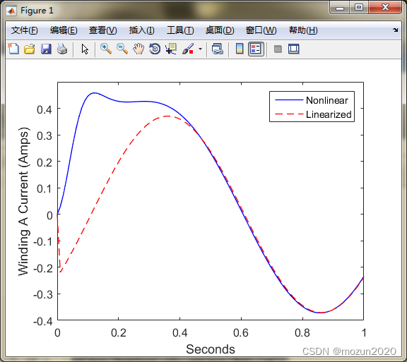
figure; hold on;
plot(tArray,xArray(1,:),'b-','LineWidth',1.0);
plot(tArray,xlinArray(1,:),'r--','LineWidth',1.0); 
set(gca,'FontSize',12); set(gcf,'Color','White'); set(gca,'Box','on');
xlabel('Seconds'); ylabel('Winding A Current (Amps)');
legend('Nonlinear', 'Linearized');

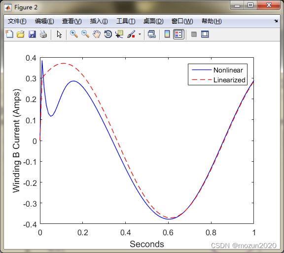
figure; hold on;
plot(tArray,xArray(2,:),'b-','LineWidth',1.0);
plot(tArray,xlinArray(2,:),'r--','LineWidth',1.0); 
set(gca,'FontSize',12); set(gcf,'Color','White'); set(gca,'Box','on');
xlabel('Seconds'); ylabel('Winding B Current (Amps)');
legend('Nonlinear', 'Linearized');

figure; hold on;
plot(tArray,xArray(3,:),'b-','LineWidth',1.0);
plot(tArray,xlinArray(3,:),'r--','LineWidth',1.0); 
set(gca,'FontSize',12); set(gcf,'Color','White'); set(gca,'Box','on');
xlabel('Seconds'); ylabel('Rotor Speed (Rad / Sec)');
legend('Nonlinear', 'Linearized');

figure; hold on;
plot(tArray,xArray(4,:),'b-','LineWidth',1.0);
plot(tArray,xlinArray(4,:),'r--','LineWidth',1.0); 
set(gca,'FontSize',12); set(gcf,'Color','White'); set(gca,'Box','on');
xlabel('Seconds'); ylabel('Rotor Position (Radians)');
legend('Nonlinear', 'Linearized');

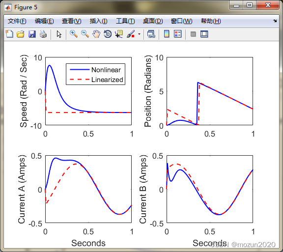
% Put all four plots in a single figure
figure;
set(gcf,'Color','White'); 

subplot(2,2,1); hold on;
plot(tArray,xArray(3,:),'b-','LineWidth',1.5);
plot(tArray,xlinArray(3,:),'r--','LineWidth',1.5); 
set(gca,'FontSize',12); set(gca,'Box','on');
ylabel('Speed (Rad / Sec)');
legend('Nonlinear', 'Linearized');

subplot(2,2,2); hold on;
plot(tArray,xArray(4,:),'b-','LineWidth',1.5);
plot(tArray,xlinArray(4,:),'r--','LineWidth',1.5); 
set(gca,'FontSize',12); set(gca,'Box','on');
ylabel('Position (Radians)');

subplot(2,2,3); hold on;
plot(tArray,xArray(1,:),'b-','LineWidth',1.5);
plot(tArray,xlinArray(1,:),'r--','LineWidth',1.5); 
set(gca,'FontSize',12); set(gca,'Box','on');
xlabel('Seconds'); ylabel('Current A (Amps)');

subplot(2,2,4); hold on;
plot(tArray,xArray(2,:),'b-','LineWidth',1.5);
plot(tArray,xlinArray(2,:),'r--','LineWidth',1.5); 
set(gca,'FontSize',12); set(gca,'Box','on');
xlabel('Seconds'); ylabel('Current B (Amps)');

2. MATLAB仿真二：示例1.3

%%%%%%%%%%%%%%%%%%%%%%%%%%%%%%%%%%%%%%%%%%%%%%%%%%%%
%功能：《最优状态估计-卡尔曼，H∞及非线性滤波》示例仿真
%示例1.3: LinearSimEx1.m
%环境：Win7，Matlab2015b
%Modi: C.S
%时间：2022-05-02
%%%%%%%%%%%%%%%%%%%%%%%%%%%%%%%%%%%%%%%%%%%%%%%%%%%%

function LinearSimEx1

% Compare rectangular, trapezoidal, and fourth order Runge Kutta integration.
% Integrate xdot = cos(t).

tf = 1;
TArray = [0.1 0.05 0.025];
for i = 1 : length(TArray)
    T = TArray(i);
    % Rectangular integration
    j = 1;
    xRect(j) = 0;
    for t = 0 : T : tf - T + T/10
        j = j + 1;
        xRect(j) = xRect(j-1) + cos(t) * T;
    end
    % Trapezoidal integration
    j = 1;
    xTrap(j) = 0;
    for t = 0 : T : tf - T + T/10
        j = j + 1;
        xTrap(j) = xTrap(j-1) + (cos(t) + cos(t+T)) * T / 2;
    end
    % Fourth order Runge Kutta integration
    j = 1;
    xRK(j) = 0;
    for t = 0 : T : tf - T + T/10
        t1 = t + T/2;
        d1 = cos(t);
        d2 = cos(t1);
        d3 = cos(t1);
        d4 = cos(t+T);
        j = j + 1;
        xRK(j) = xRK(j-1) + (d1 + 2 * d2 + 2 * d3 + d4) * T / 6;
    end
    errRect = 100 * abs(xRect(end) - sin(tf)) / sin(tf);
    errTrap = 100 * abs(xTrap(end) - sin(tf)) / sin(tf);
    errRK = 100 * abs(xRK(end) - sin(tf)) / sin(tf);
    disp(['T = ', num2str(T), ': ', num2str(errRect), ', ', num2str(errTrap), ', ', num2str(errRK)]);
end

仿真结果：

>> LinearSimEx1
T = 0.1: 2.6482, 0.083347, 3.4733e-06
T = 0.05: 1.3449, 0.020834, 2.1703e-07
T = 0.025: 0.67767, 0.0052084, 1.3564e-08

3. 小结

运动控制在现代生活中的实际应用非常广泛，除了智能工厂中各种智能设备的自动运转控制，近几年最火的自动驾驶技术，以及航空航天领域，都缺少不了它的身影，所以熟练掌握状态估计理论，对未来就业也是非常有帮助的。切记矩阵理论与概率论等知识的基础一定要打好。对本章内容感兴趣或者想充分学习了解的，建议去研习书中第一章节的内容，有条件的可以通过习题的联系进一步巩固充实。后期会对其中一些知识点在自己理解的基础上进行讨论补充，欢迎大家一起学习交流。

原书链接：Optimal State Estimation:Kalman, H-infinity, and Nonlinear Approaches