YOLOV4翻译

YOLOv4: Optimal Speed and Accuracy of Object Detection

Alexey Bochkovskiy alexeyab84@gmail.com

Chien-Yao Wang Institute of Information Science Academia Sinica, Taiwan kinyiu@iis.sinica.edu.tw

Hong-Yuan Mark Liao Institute of Information Science Academia Sinica, Taiwan liao@iis.sinica.edu.tw

Abstract

There are a huge number of features which are said to improve Convolutional Neural Network (CNN) accuracy. Practical testing of combinations of such features on large datasets, and theoretical justification of the result, is required. Some features operate on certain models exclusively and for certain problems exclusively, or only for small-scale datasets; while some features, such as batch-normalization and residual-connections, are applicable to the majority of models, tasks, and datasets. We assume that such universal features include Weighted-Residual-Connections (WRC), Cross Stage-Partial-connections (CSP), Cross mini-Batch Normalization (CmBN), Self-adversarial-training (SAT) and Mish-activation. We use new features: WRC, CSP, CmBN, SAT, Mish activation, Mosaic data augmentation, CmBN, DropBlock regularization, and CIoU loss, and combine some of them to achieve state-of-the-art results: 43.5% AP (65.7% AP50) for the MS COCO dataset at a realtime speed of 65 FPS on Tesla V100. Source code is at https://github.com/AlexeyAB/darknet.

据说有大量特征可以提高卷积神经网络（CNN）的准确性。我们需要在大型数据集上对这些特征的组合进行实际测试，并对结果进行理论论证。有些特征只适用于某些模型，只适用于某些问题，或只适用于小规模数据集；而有些特征，如批次归一化和残差连接，则适用于大多数模型、任务和数据集。我们假定这些通用特征包括Weighted-Residual-Connections (WRC)、Cross Stage-Partial-connections(CSP)、 Cross mini-Batch Normalization(CmBN)、Self-adversarial-training(SAT)和Mish-activation。我们使用了新的特征：WRC、CSP、CmBN、SAT、Mish 激活、Mosaic 数据增强、CmBN、DropBlock 正则化和 CIoU 损失，并将其中一些功能结合起来，以达到 state-of-the-art 效果： 在Tesla V100 上以 65 FPS 的实时速度处理 MS COCO 数据集时，AP 为 43.5%（AP50 为 65.7%）。源代码见 https://github.com/AlexeyAB/darknet。

1 Introduction

The majority of CNN-based object detectors are largely applicable only for recommendation systems. For example, searching for free parking spaces via urban video cameras is executed by slow accurate models, whereas car collision warning is related to fast inaccurate models. Improving the real-time object detector accuracy enables using them not only for hint generating recommendation systems, but also for stand-alone process management and human input reduction. Real-time object detector operation on conventional Graphics Processing Units (GPU) allows their mass usage at an affordable price. The most accurate modern neural networks do not operate in real time and require large number of GPUs for training with a large mini-batch-size. We address such problems through creating a CNN that operates in real-time on a conventional GPU, and for which training requires only one conventional GPU.

大多数基于 CNN 的目标检测器在很大程度上只适用于推荐系统。例如，通过城市视频摄像头搜索空闲停车位是由慢速精确模型执行的，而汽车碰撞预警则与快速不精确模型有关。提高实时目标检测器的精确度，不仅能将其用于生成提示的推荐系统，还能用于独立的流程管理和减少人工输入。在传统图形处理器（GPU）上运行实时目标检测器，能以合理的价格大规模使用。最精确的现代神经网络无法实时运行，需要大量 GPU 进行小批量训练。为了解决这些问题，我们创建了一个可在传统 GPU 上实时运行的 CNN，其训练只需要一个传统 GPU。

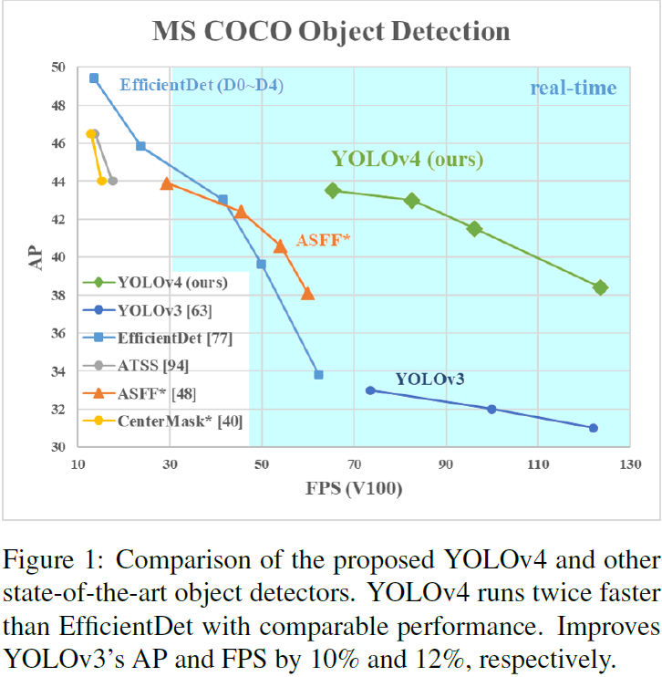
The main goal of this work is designing a fast operating speed of an object detector in production systems and optimization for parallel computations, rather than the low computation volume theoretical indicator (BFLOP). We hope that the designed object can be easily trained and used. For example, anyone who uses a conventional GPU to train and test can achieve real-time, high quality, and convincing object detection results, as the YOLOv4 results shown in Figure 1. Our contributions are summarized as follows:

这项工作的主要目标是设计用于生产系统中能够快速运行的目标检测器，并针对并行计算进行优化，而不是为了降低计算量理论指标（BFLOP）。我们希望所设计的目标模型可以很容易地训练和使用。例如，任何人使用传统 GPU 进行训练和检测，都能获得实时、高质量、令人信服的目标检测结果，如图 1 所示的 YOLOv4 结果。 我们的贡献总结如下：

1. We develope an efficient and powerful object detection model. It makes everyone can use a 1080 Ti or 2080 Ti GPU to train a super fast and accurate object detector.

   我们开发了一个高效、强大的目标检测模型。它使每个人都能使用 1080 Ti 或 2080 Ti GPU 训练出超快、超准的目标检测器。

2. We verify the influence of state-of-the-art Bag-of-Freebies and Bag-of-Specials methods of object detection during the detector training.

   在检测器训练过程中，我们验证了最先进的Bag-of-Freebies和 Bag-of-Specials目标检测方法的影响。

3. We modify state-of-the-art methods and make them more effecient and suitable for single GPU training, including CBN [89], PAN [49], SAM [85], etc.

   我们修改了最先进的方法，使其更加高效并适合单 GPU 训练，包括 CBN [89]、PAN [49]、SAM [85] 等。

2 Related work

2.1 Object detection models

A modern detector is usually composed of two parts, a backbone which is pre-trained on ImageNet and a head which is used to predict classes and bounding boxes of objects. For those detectors running on GPU platform, their backbone could be VGG [68], ResNet [26], ResNeXt [86], or DenseNet [30]. For those detectors running on CPU platform, their backbone could be SqueezeNet [31], MobileNet [28, 66, 27, 74], or ShuffleNet [97, 53]. As to the head part, it is usually categorized into two kinds, i.e., one-stage object detector and two-stage object detector. The most representative two-stage object detector is the R-CNN [19] series, including fast R-CNN [18], faster R-CNN [64], R-FCN [9], and Libra R-CNN [58]. It is also possible to make a twostage object detector an anchor-free object detector, such as RepPoints [87]. As for one-stage object detector, the most representative models are YOLO [61, 62, 63], SSD [50], and RetinaNet [45]. In recent years, anchor-free one-stage object detectors are developed. The detectors of this sort are CenterNet [13], CornerNet [37, 38], FCOS [78], etc. Object detectors developed in recent years often insert some layers between backbone and head, and these layers are usually used to collect feature maps from different stages. We can call it the neck of an object detector. Usually, a neck is composed of several bottom-up paths and several top down paths. Networks equipped with this mechanism include Feature Pyramid Network (FPN) [44], Path Aggregation Network (PAN) [49], BiFPN [77], and NAS-FPN [17].In addition to the above models, some researchers put their emphasis on directly building a new backbone (DetNet [43], DetNAS [7]) or a new whole model (SpineNet [12], HitDetector [20]) for object detection.

现代检测器通常由两部分组成，一部分是在 ImageNet 上预先训练好的backbone，另一部分是用于预测物体类别和边界框的Header。对于在 GPU 平台上运行的检测器，其主干可以是 VGG [68]、ResNet [26]、ResNeXt [86] 或 DenseNet [30]。至于在 CPU 平台上运行的检测器，其骨干网可以是 SqueezeNet [31]、MobileNet [28, 66, 27, 74] 或 ShuffleNet [97, 53]。至于Header部分，通常分为两类，即单级(one-stage)目标检测器和两级(two-stage)目标检测器。最具代表性的two-stage目标检测器是 R-CNN [19] 系列，包括 fast R-CNN [18]、faster R-CNN [64]、R-FCN [9] 和 Libra R-CNN [58]。也可以将两阶段目标检测器做成无锚目标检测器，如 RepPoints [87]。至于单级(one-stage)目标检测器，最具代表性的模型有 YOLO [61, 62, 63]、SSD [50] 和 RetinaNet [45]。近年来，无锚单级目标检测器(anchor-free one-stage object detectors)也得到了发展。这类检测器有 CenterNet [13]、CornerNet [37, 38]、FCOS [78] 等。近年来开发的目标检测器往往在骨干和头部之间插入一些层，这些层通常用来收集不同阶段的特征图。我们可以称其为目标检测器的颈部(neck )。通常，颈部由几条自下而上的路径和几条自上而下的路径组成。具备这种机制的网络包括特征金字塔网络（FPN）[44]、路径聚合网络（PAN）[49]、BiFPN[77]和 NAS-FPN[17]。除上述模型外，一些研究者还将重点放在直接构建新的骨干网（DetNet [43]、DetNAS [7]）或新的整体模型（SpineNet [12]、HitDetector [20]）来进行目标检测上。

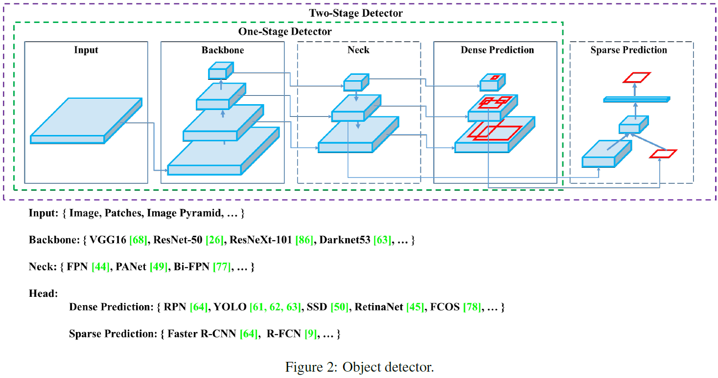
To sum up, an ordinary object detector is composed of
several parts:

• Input: Image, Patches, Image Pyramid

• Backbones: VGG16 [68], ResNet-50 [26], SpineNet [12], EfficientNet-B0/B7 [75], CSPResNeXt50 [81], CSPDarknet53 [81]

• Neck:

• Additional blocks: SPP [25], ASPP [5], RFB [47], SAM [85]

• Path-aggregation blocks: FPN [44], PAN [49], NAS-FPN [17], Fully-connected FPN, BiFPN [77], ASFF [48], SFAM [98]

• Heads:

• Dense Prediction (one-stage):
  - RPN [64], SSD [50], YOLO [61], RetinaNet [45] (anchor based)
  - CornerNet [37], CenterNet [13], MatrixNet [60], FCOS [78] (anchor free)

• Sparse Prediction (two-stage):
  - Faster R-CNN [64], R-FCN [9], Mask RCNN [23] (anchor based)
  - RepPoints [87] (anchor free)

总之，普通的目标检测器由以下几个部分组成
几个部分组成：

• 输入 图像、patches、图像金字塔

• Backbones： VGG16[68]、ResNet-50[26]、SpineNet[12]、EfficientNet-B0/B7[75]、CSPResNeXt50[81]、CSPDarknet53[81]。

• Neck：

  • 附加区块： SPP[25]、ASP[5]、RFB[47]、SAM[85]
  • 路径聚合区块： FPN[44]、PAN[49]、NAS-FPN[17]、全连接 FPN、BiFPN[77]、ASFF[48]、SFAM[98]

• Header

  • 密集预测（one stage）：
    • RPN [64]、SSD [50]、YOLO [61]、RetinaNet [45]（基于锚点）
    • CornerNet [37]、CenterNet [13]、MatrixNet [60]、FCOS [78]（无锚点）
  • 稀疏预测（two stage）：
    • 更快的 R-CNN [64]、R-FCN [9]、掩码 RCNN [23] （基于锚点）
    • RepPoints [87] （无锚点）

2.2. Bag of freebies

Usually, a conventional object detector is trained offline. Therefore, researchers always like to take this advantage and develop better training methods which can make the object detector receive better accuracy without increasing the inference cost. We call these methods that only change the training strategy or only increase the training cost as “bag of freebies.” What is often adopted by object detection methods and meets the definition of bag of freebies is data augmentation. The purpose of data augmentation is to increase the variability of the input images, so that the designed object detection model has higher robustness to the images obtained from different environments. For examples, photometric distortions and geometric distortions are two commonly used data augmentation method and they definitely benefit the object detection task. In dealing with photometric distortion, we adjust the brightness, contrast, hue, saturation, and noise of an image. For geometric distortion, we add random scaling, cropping, flipping, and rotating.

通常，传统的目标检测器是离线训练的。因此，研究人员总是喜欢利用这一优势，开发出更好的训练方法，在不增加推理成本的情况下，使目标检测器获得更高的精度。我们把这些只改变训练策略或只增加训练成本的方法称为 “bag of freebies”。物体检测方法经常采用的、符合bag of freebies定义的方法是数据增强。数据增强的目的是增加输入图像的可变性，从而使设计的目标检测模型对不同环境下获得的图像具有更高的鲁棒性。例如，光度畸变和几何畸变是两种常用的数据增强方法，它们无疑对目标检测任务大有裨益。在处理光度失真时，我们会调整图像的亮度、对比度、色调、饱和度和噪点。对于几何失真，我们会添加随机缩放、裁剪、翻转和旋转。

The data augmentation methods mentioned above are all pixel-wise adjustments, and all original pixel information in the adjusted area is retained. In addition, some researchers engaged in data augmentation put their emphasis on simulating object occlusion issues. They have achieved good results in image classification and object detection. For example, random erase [100] and Cut-Out [11] can randomly select the rectangle region in an image and fill in a random or complementary value of zero. As for hide-and-seek [69] and grid mask [6], they randomly or evenly select multiple rectangle regions in an image and replace them to all zeros. If similar concepts are applied to feature maps, there are Drop-Out [71], Drop-Connect [80], and Drop-Block [16] methods. In addition, some researchers have proposed the methods of using multiple images together to perform data augmentation. For example, Mix-Up [92] uses two images to multiply and superimpose with different coefficient ratios, and then adjusts the label with these superimposed ratios. As for Cut-Mix [91], it is to cover the cropped image to rectangle region of other images, and adjusts the label according to the size of the mix area. In addition to the above mentioned methods, style transfer GAN [15] is also used for data augmentation, and such usage can effectively reduce the texture bias learned by CNN.

上述数据增强方法都是像素级调整，调整区域内的所有原始像素信息都会保留。此外，一些从事数据增强的研究人员将重点放在模拟物体遮挡问题上。他们在图像分类和目标检测方面取得了不错的成果。例如，随机擦除法(random erase)[100]和剪切法(Cut-out)[11]可以随机选择图像中的矩形区域，并填充一个随机值或补零值。至于hide-and-seek[69]和网格掩码(grid mask)[6]，它们会随机或均匀地选择图像中的多个矩形区域，并将其替换为全部零。如果将类似的概念应用于特征图，则有 Drop-Out [71]、Drop-Connect [80] 和 Drop-Block [16] 等方法。此外，一些研究人员还提出了将多幅图像结合在一起进行数据增强的方法。例如，Mix-Up[92] 使用两幅图像以不同的系数比例相乘叠加，然后根据这些叠加比例调整标签。至于 Cut-Mix [91]，则是将裁剪后的图像覆盖到其他图像的矩形区域，并根据混合区域的大小调整标签。除上述方法外，style transfer GAN [15] 也被用于数据增强，这种用法可以有效减少 CNN 学习到的纹理偏差。

Different from the various approaches proposed above, some other bag of freebies methods are dedicated to solving the problem that the semantic distribution in the dataset may have bias. In dealing with the problem of semantic distribution bias, a very important issue is that there is a problem of data imbalance between different classes, and this problem is often solved by hard negative example mining [72] or online hard example mining [67] in two-stage object detector. But the example mining method is not applicable to one-stage object detector, because this kind of detector belongs to the dense prediction architecture. Therefore Lin et al. [45] proposed focal loss to deal with the problem of data imbalance existing between various classes. Another very important issue is that it is difficult to express the relationship of the degree of association between different categories with the one-hot hard representation. This representation scheme is often used when executing labeling. The label smoothing proposed in [73] is to convert hard label into soft label for training, which can make model more robust. In order to obtain a better soft label, Islam et al. [33] introduced the concept of knowledge distillation to design the label refinement network.

与上述提出的各种方法不同，其他一些bag of freebies致力于解决数据集中的语义分布可能存在偏差的问题。在处理语义分布偏差问题时，一个非常重要的问题是不同类之间存在数据不平衡的问题，这个问题通常是通过两阶段目标检测器中的负样本难例挖掘(hard negative example mining, HEM)[72]或在线难例挖掘(online hard example mining, OHEM)[67]来解决的。但实例挖掘方法不适用于单级目标检测器，因为这类检测器属于密集预测架构。因此，Lin 等人[45]提出了焦点损失法（focal loss）来处理不同类别之间存在的数据不平衡问题。另一个非常重要的问题是，one-hot表示法很难表达不同类别之间的关联程度关系。这种表示方案通常在执行标签时使用。文献[73]中提出的标签平滑法(label smoothing)是将硬标签转换为软标签进行训练，这样可以使模型更加robust。为了获得更好的软标签，Islam等人[33]引入了知识蒸馏(concept of knowledge distillation)来设计标签细化网络。

The last bag of freebies is the objective function of Bounding Box (BBox) regression. The traditional object detector usually uses Mean Square Error (MSE) to directly perform regression on the center point coordinates and height and width of the BBox, i.e., { x c e n t e r , y c e n t e r , w , h } \{x_{center}, y_{center}, w, h\} {xcenter​,ycenter​,w,h}, or the upper left point and the lower right point, i.e., { x t o p _ l e f t , y t o p _ l e f t , x b o t t o m _ r i g h t , y b o t t o m _ r i g h t g } \{x_{top\_left}, y_{top\_left}, x_{bottom\_right}, y_{bottom\_rightg}\} {xtop_left​,ytop_left​,xbottom_right​,ybottom_rightg​}. As for anchor-based method, it is to estimate the corresponding offset, for example { x c e n t e r _ o f f s e t , y c e n t e r _ o f f s e t , w o f f s e t , h o f f s e t } \{x_{center\_offset}, y_{center\_offset}, w_{offset}, h_{offset}\} {xcenter_offset​,ycenter_offset​,woffset​,hoffset​} and { x t o p _ l e f t _ o f f s e t , y t o p _ l e f t _ o f f s e t , x b o t t o m _ r i g h t _ o f f s e t , y b o t t o m _ r i g h t _ o f f s e t g } \{x_{top\_left\_offset}, y_{top\_left\_offset}, x_{bottom\_right\_offset}, y_{bottom\_right\_offsetg}\} {xtop_left_offset​,ytop_left_offset​,xbottom_right_offset​,ybottom_right_offsetg​} . However, to directly estimate the coordinate values of each point of the BBox is to treat these points as independent variables, but in fact does not consider the integrity of the object itself. In order to make this issue processed better, some researchers recently proposed IoU loss [90], which puts the coverage of predicted BBox area and ground truth BBox area into consideration. The IoU loss computing process will trigger the calculation of the four coordinate points of the BBox by executing IoU with the ground truth, and then connecting the generated results into a whole code. Because IoU is a scale invariant representation, it can solve the problem that when traditional methods calculate the l1 or l2 loss of { x , y , w , h } \{x, y, w, h\} {x,y,w,h}, the loss will increase with the scale. Recently, some researchers have continued to improve IoU loss. For example, GIoU loss [65] is to include the shape and orientation of object in addition to the coverage area. They proposed to find the smallest area BBox that can simultaneously cover the predicted BBox and ground truth BBox, and use this BBox as the denominator to replace the denominator originally used in IoU loss. As for DIoU loss [99], it additionally considers the distance of the center of an object, and CIoU loss [99], on the other hand simultaneously considers the overlapping area, the distance between center points, and the aspect ratio. CIoU can achieve better convergence speed and accuracy on the BBox regression problem.

最后一个Bag_of_freebies是边框箱（BBox）回归的目标函数。传统的目标检测器通常使用均方误差（MSE）直接对 BBox 的中心点坐标和高度、宽度进行回归，即 { x c e n t e r , y c e n t e r , w , h } \{x_{center}, y_{center}, w, h\} {xcenter​,ycenter​,w,h} 或者左上点和右下点，即 { x t o p _ l e f t , y t o p _ l e f t , x b o t t o m _ r i g h t , y b o t t o m _ r i g h t g } \{x_{top\_left}, y_{top\_left}, x_{bottom\_right}, y_{bottom\_rightg}\} {xtop_left​,ytop_left​,xbottom_right​,ybottom_rightg​} 。至于基于锚点的方法，则是估计相应的偏移量，例如 { x c e n t e r _ o f f s e t , y c e n t e r _ o f f s e t , w o f f s e t , h o f f s e t } \{x_{center\_offset}, y_{center\_offset}, w_{offset}, h_{offset}\} {xcenter_offset​,ycenter_offset​,woffset​,hoffset​} 和 { x t o p _ l e f t _ o f f s e t , y t o p _ l e f t _ o f f s e t , x b o t t o m _ r i g h t _ o f f s e t , y b o t t o m _ r i g h t _ o f f s e t g } \{x_{top\_left\_offset}, y_{top\_left\_offset}, x_{bottom\_right\_offset}, y_{bottom\_right\_offsetg}\} {xtop_left_offset​,ytop_left_offset​,xbottom_right_offset​,ybottom_right_offsetg​} 。然而，直接估计 BBox 中每个点的坐标值是将这些点视为独立变量，但实际上并没有考虑对象本身的完整性。为了使这个问题得到更好的处理，一些研究人员最近提出了 IoU loss [90]，将预测 BBox 区域和 ground truth BBox 区域的覆盖率纳入考虑范围。IoU 损失计算过程将通过执行 IoU 与ground truth的四个坐标点的计算，然后将生成的结果连接成一个整体。由于 IoU 是一种尺度不变表示法，它可以解决传统方法计算 { x 、 y 、 w 、 h } \{x、y、w、h\} {x、y、w、h} 的 L1 或 L2 损失时，损失会随尺度增大而增大的问题。最近，一些研究人员不断改进 IoU loss。例如，GIoU loss[65]是在覆盖范围之外再加上物体的形状和方向。他们提出找到能同时覆盖预测 BBox 和 ground truth BBox 的最小区域 BBox，并以此 BBox 为分母，取代 IoU loss 最初使用的分母。DIoU loss [99]则额外考虑了物体中心的距离，而 CIoU loss [99]则同时考虑了重叠区域、中心点之间的距离和长宽比。在 BBox 回归问题上，CIoU 可以达到更好的收敛速度和精度。

2.3. Bag of specials

For those plugin modules and post-processing methods that only increase the inference cost by a small amount but can significantly improve the accuracy of object detection, we call them “bag of specials”. Generally speaking, these plugin modules are for enhancing certain attributes in a model, such as enlarging receptive field, introducing attention mechanism, or strengthening feature integration capability, etc., and post-processing is a method for screening model prediction results.

对于那些只增加少量推理成本，却能显著提高目标检测精度的插件模块和后处理方法，我们称之为 “Bag Of Specials”。一般来说，这些插件模块用于增强模型的某些属性，如扩大感受野、引入注意机制或加强特征整合能力等，而后处理则是筛选模型预测结果的一种方法。

Common modules that can be used to enhance receptive field are SPP [25], ASPP [5], and RFB [47]. The SPP module was originated from Spatial Pyramid Matching(SPM) [39], and SPMs original method was to split feature map into several $d\times d$ equal blocks, where $d$ can be {1; 2; 3; ……}, thus forming spatial pyramid, and then extracting bag-of-word features. SPP integrates SPM into CNN and use max-pooling operation instead of bag-of-word operation. Since the SPP module proposed by He et al. [25] will output one dimensional feature vector, it is infeasible to be applied in Fully Convolutional Network (FCN). Thus in the design of YOLOv3 [63], Redmon and Farhadi improve SPP module to the concatenation of max-pooling outputs with kernel size $k\times k$, where k = { 1 , 5 , 9 , 13 } k = \{1,5,9,13\} k={1,5,9,13}, and stride equals to 1. Under this design, a relatively large $k\times k$ maxpooling effectively increase the receptive field of backbone feature. After adding the improved version of SPP module, YOLOv3-608 upgrades $A{P}_{50}$ by 2.7% on the MS COCO object detection task at the cost of 0.5% extra computation. The difference in operation between ASPP [5] module and improved SPP module is mainly from the original $k\times k$ kernel size, max-pooling of stride equals to 1 to several $3\times 3$ kernel size, dilated ratio equals to $k$, and stride equals to 1 in dilated convolution operation. RFB module is to use several dilated convolutions of $k\times k$ kernel, dilated ratio equals to $k$, and stride equals to 1 to obtain a more comprehensive spatial coverage than ASPP. RFB [47] only costs 7% extra inference time to increase the AP50 of SSD on MS COCO by 5.7%.

可用于增强感受野的常见模块有 SPP [25]、ASPP [5] 和 RFB [47]。SPP 模块源于空间金字塔匹配（Spatial Pyramid Matching，SPM）[39]，SPM 的原始方法是将特征图分割成若干个 $d\times d$ 相等的块，其中 $d$ 可以是 {1,2, 3, …}，从而形成空间金字塔，然后提取bag-of-word特征。SPP 将 SPM 集成到 CNN 中，使用 max-pooling 运算代替bag-of-word运算。由于 He 等人[25]提出的 SPP 模块将输出一维特征向量，因此无法应用于全卷积网络（FCN）。因此，在 YOLOv3 [63] 的设计中，Redmon 和 Farhadi 将 SPP 模块改进为最大池化输出的串联，内核大小为 $k\times k$，其中 k = { 1 , 5 , 9 , 13 } k = \{1,5,9,13\} k={1,5,9,13}，步长等于 1。在这种设计下，相对较大的 $k\times k$ max-pooling 能有效增加主干特征的感受野。在添加改进版 SPP 模块后，YOLOv3-608 在 MS COCO 目标检测任务上将 $A{P}_{50}$ 提升了 2.7%，而代价是额外增加了 0.5% 的计算量。ASPP[5]模块与改进后的SPP模块在操作上的差异主要是从原来的$k\times k$内核大小、最大池化步长等于1到多个$3\times 3$内核大小、扩张比(dilated ratio)等于k，dilated convolution操作中步长等于1。RFB 模块是使用若干个 $k\times k$ 内核，扩张比(dilated ratio)等于 k，步长等于 1 的dilated convolution，以获得比 ASPP 更全面的空间覆盖。RFB[47]只花费了 7% 的额外推理时间，就能将 SSD 在 MS COCO 上的 AP50 提高 5.7%。

The attention module that is often used in object detection is mainly divided into channel-wise attention and pointwise attention, and the representatives of these two attention models are Squeeze-and-Excitation (SE) [29] and Spatial Attention Module (SAM) [85], respectively. Although SE module can improve the power of ResNet50 in the ImageNet image classification task 1% top-1 accuracy at the cost of only increasing the computational effort by 2%, but on a GPU usually it will increase the inference time by about 10%, so it is more appropriate to be used in mobile devices. But for SAM, it only needs to pay 0.1% extra calculation and it can improve ResNet50-SE 0.5% top-1 accuracy on the ImageNet image classification task. Best of all, it does not affect the speed of inference on the GPU at all.

在目标检测中经常使用的注意模块主要分为channel-wise attention 和pointwise attention，这两种注意模型的代表分别是 Squeeze-and-Excitation(SE）[29]和Spatial Attention Module(SAM)[85]。虽然 SE 模块可以提高 ResNet50 在 ImageNet 图像分类任务中 1% top-1 的准确率，而代价只是增加 2% 的计算量，但在 GPU 上通常会增加 10% 左右的推理时间，因此更适合在移动设备上使用。但对于 SAM 来说，它只需要付出 0.1% 的额外计算量，就能在 ImageNet 图像分类任务中将 ResNet50-SE 的 top-1 准确率提高 0.5%。最重要的是，它完全不会影响 GPU 的推理速度。

In terms of feature integration, the early practice is to use skip connection [51] or hyper-column [22] to integrate low level physical feature to high-level semantic feature. Since multi-scale prediction methods such as FPN have become popular, many lightweight modules that integrate different feature pyramid have been proposed. The modules of this sort include SFAM [98], ASFF [48], and BiFPN [77]. The main idea of SFAM is to use SE module to execute channel wise level re-weighting on multi-scale concatenated feature maps. As for ASFF, it uses softmax as point-wise level reweighting and then adds feature maps of different scales. In BiFPN, the multi-input weighted residual connections is proposed to execute scale-wise level re-weighting, and then add feature maps of different scales.

在特征整合方面，早期的做法是利用skip connection[51]或 hyper-column[22]将低层次的物理特征整合到高层次的语义特征中。自 FPN 等多尺度预测方法流行以来，许多集成不同特征金字塔的轻量级模块被提出。这类模块包括 SFAM [98]、ASFF [48] 和 BiFPN [77]。SFAM 的主要思想是使用 SE 模块对多尺度串联特征图进行信道级再加权。至于 ASFF，它使用 softmax 作为点向级再加权，然后添加不同尺度的特征图。在 BiFPN 中，提出了多输入加权残差连接来执行按比例的水平再加权，然后添加不同比例的特征图。

In the research of deep learning, some people put their focus on searching for good activation function. A good activation function can make the gradient more efficiently propagated, and at the same time it will not cause too much extra computational cost. In 2010, Nair and Hinton [56] propose ReLU to substantially solve the gradient vanish problem which is frequently encountered in traditional tanh and sigmoid activation function. Subsequently, LReLU [54], PReLU [24], ReLU6 [28], Scaled Exponential Linear Unit (SELU) [35], Swish [59], hard-Swish [27], and Mish [55], etc., which are also used to solve the gradient vanish problem, have been proposed. The main purpose of LReLU and PReLU is to solve the problem that the gradient of ReLU is zero when the output is less than zero. As for ReLU6 and hard-Swish, they are specially designed for quantization networks. For self-normalizing a neural network, the SELU activation function is proposed to satisfy the goal. One thing to be noted is that both Swish and Mish are continuously differentiable activation function.

在深度学习的研究中，有人把重点放在寻找好的激活函数上。一个好的激活函数可以使梯度更有效地传播，同时也不会带来太多额外的计算成本。2010 年，Nair 和 Hinton[56]提出了 ReLU，大大解决了传统 tanh 和 sigmoid 激活函数经常遇到的梯度消失问题。随后，同样用于解决梯度消失问题的 LReLU [54]、PReLU [24]、ReLU6 [28]、Scale Exponential Linear Unit（SELU）[35]、Swish [59]、hard-Swish [27] 和 Mish [55] 等也相继被提出。LReLU 和 PReLU 的主要目的是解决当输出小于零时 ReLU 梯度为零的问题。至于 ReLU6 和 hard-Swish，它们是专门为量化网络设计的。为了实现神经网络的自规范化，提出了 SELU 激活函数来满足这一目标。值得注意的是，Swish 和 Mish 都是连续可微的激活函数。

The post-processing method commonly used in deeplearning-based object detection is NMS, which can be used to filter those BBoxes that badly predict the same object, and only retain the candidate BBoxes with higher response. The way NMS tries to improve is consistent with the method of optimizing an objective function. The original method proposed by NMS does not consider the context information, so Girshick et al. [19] added classification confidence score in R-CNN as a reference, and according to the order of confidence score, greedy NMS was performed in the order of high score to low score. As for soft NMS [1], it considers the problem that the occlusion of an object may cause the degradation of confidence score in greedy NMS with IoU score. The DIoU NMS [99] developers way of thinking is to add the information of the center point distance to the BBox screening process on the basis of soft NMS. It is worth mentioning that, since none of above postprocessing methods directly refer to the captured image features, post-processing is no longer required in the subsequent development of an anchor-free method.

基于深度学习的目标检测中常用的后处理方法是 NMS，它可以用来过滤那些对同一目标预测不好的 BBox，只保留响应较高的候选 BBox。NMS 尝试改进的方式与优化目标函数的方法一致。NMS 最初提出的方法没有考虑上下文信息，因此 Girshick 等人[19]加入了 R-CNN 中的分类置信度得分作为参考，根据置信度得分的高低，按照从高分到低分的顺序进行贪婪 NMS。至于软 NMS [1]，它考虑到了物体遮挡可能会导致 IoU 分数的贪婪 NMS 中置信度分数下降的问题。DIoU NMS [99] 的开发思路是在软 NMS 的基础上，在 BBox 筛选过程中加入中心点距离信息。值得一提的是，由于上述后处理方法都不直接参考捕捉到的图像特征，因此在无锚点方法的后续开发中不再需要后处理。

3 Methodology

The basic aim is fast operating speed of neural network, in production systems and optimization for parallel computations, rather than the low computation volume theoretical indicator (BFLOP). We present two options of real-time neural networks:

其基本目标是在生产系统和并行计算优化中实现神经网络的快速运行速度，而不是低计算量理论指标（BFLOP）。我们提出了两种实时神经网络：

• For GPU we use a small number of groups (1 - 8) in convolutional layers: CSPResNeXt50 / CSPDarknet53

  对于 GPU，我们在卷积层中使用少量组（1 - 8）： CSPResNeXt50 / CSPDarknet53

• For VPU - we use grouped-convolution, but we refrain from using Squeeze-and-excitement (SE) blocks specifically this includes the following models: EfficientNet-lite / MixNet [76] / GhostNet [21] / MobileNetV3

  对于 VPU，我们使用分组卷积，但不使用SE块，具体包括以下模型：EfficientNet-lite、MixNet [76]、GhostNet [21] 、MobileNetV3

3.1. Selection of architecture

Our objective is to find the optimal balance among the input network resolution, the convolutional layer number, the parameter number $(filter\_siz{e}^2\ast filters\ast channel/groups)$, and the number of layer outputs (filters). For instance, our numerous studies demonstrate that the CSPResNext50 is considerably better compared to CSPDarknet53 in terms of object classification on the ILSVRC2012 (ImageNet) dataset [10]. However, conversely, the CSPDarknet53 is better compared to CSPResNext50 in terms of detecting objects on the MS COCO dataset [46].

我们的目标是在输入网络分辨率、卷积层数、参数数 $(filter\_siz{e}^2\ast filters\ast channel/groups)$ 和层输出（过滤器）数之间找到最佳平衡。例如，我们的大量研究表明，与 CSPDarknet53 相比，CSPResNext50 在 ILSVRC2012（ImageNet）数据集的对象分类方面要好得多[10]。不过，反过来说，CSPDarknet53 与 CSPResNext50 相比 CSPResNext50在 MS COCO 数据集[46]上的目标检测能力更强。

The next objective is to select additional blocks for increasing the receptive field and the best method of parameter aggregation from different backbone levels for different detector levels: e.g. FPN, PAN, ASFF, BiFPN.

下一个目标是针对不同的检测器级别：如 FPN、PAN、ASFF、BiFPN，从不同的骨干网级别中选择增加感受野的附加区块和参数聚合的最佳方法。

A reference model which is optimal for classification is not always optimal for a detector. In contrast to the classifier, the detector requires the following:

对分类最优的参考模型不一定对检测器最优。与分类器相比，检测器需要具备以下条件：

• Higher input network size (resolution) – for detecting multiple small-sized objects
• More layers – for a higher receptive field to cover the increased size of input network
• More parameters – for greater capacity of a model to detect multiple objects of different sizes in a single image
• 更高的输入网络规模（分辨率）–用于检测多个小尺寸目标
• 层数更多–以更高的感受野覆盖更大的输入网络
• 更多参数–使模型更有能力检测单幅图像中不同大小的多个目标

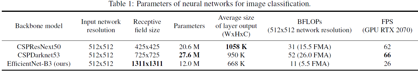
Hypothetically speaking, we can assume that a model with a larger receptive field size (with a larger number of convolutional layers $3\times 3$) and a larger number of parameters should be selected as the backbone. Table 1 shows the information of CSPResNeXt50, CSPDarknet53, and EfficientNet B3. The CSPResNext50 contains only 16 convolutional layers $3\times 3$, a $425\times 425$ receptive field and 20.6M parameters, while CSPDarknet53 contains 29 convolutional layers $3\times 3$, a $725\times 725$ receptive field and 27.6M parameters. This theoretical justification, together with our numerous experiments, show that CSPDarknet53 neural network is the optimal model of the two as the backbone for a detector.

从假设上讲，我们可以认为应该选择一个具有更大感受野（卷积层数为 $3\times 3$）和更多参数的模型作为主干。表 1 列出了 CSPResNeXt50、CSPDarknet53 和 EfficientNet B3 的信息。CSPResNext50 只包含 16 个卷积层，$3\times 3$ ，$425 \times 425 $的感受野和 20.6M参数；而 CSPDarknet53 包含 29 个卷积层，$3\times 3$，725 ×725 次的感受野和 27.60M参数。这一理论依据以及我们的大量实验表明，CSPDarknet53 神经网络是两者中作为探测器骨干的最佳模型。

• The influence of the receptive field with different sizes is summarized as follows: Up to the object size - allows viewing the entire object

  不同大小的感受野的影响总结如下：达到物体大小–可观察整个物体

• Up to network size - allows viewing the context around the object

达到网络尺寸–可查看物体周围的环境

• Exceeding the network size - increases the number of connections between the image point and the final activation

超过网络大小–增加图像点和最终激活之间的连接数量

We add the SPP block over the CSPDarknet53, since it significantly increases the receptive field, separates out the most significant context features and causes almost no reduction of the network operation speed. We use PANet as the method of parameter aggregation from different backbone levels for different detector levels, instead of the FPN used in YOLOv3.

我们在 CSPDarknet53 的基础上添加了 SPP 块，因为它能显著增加感受野，分离出最重要的上下文特征，而且几乎不会降低网络运行速度。我们使用 PANet 作为不同检测器级别的不同骨干层的参数聚合方法，而不是 YOLOv3 中使用的 FPN。

Finally, we choose CSPDarknet53 backbone, SPP additional module, PANet path-aggregation neck, and YOLOv3 (anchor based) head as the architecture of YOLOv4. In the future we plan to expand significantly the content of Bag of Freebies (BoF) for the detector, which theoretically can address some problems and increase the detector accuracy, and sequentially check the influence of each feature in an experimental fashion.

最后，我们选择 CSPDarknet53 主干网、SPP 附加模块、PANet 路径聚合颈和 YOLOv3（基于锚）头作为 YOLOv4 的架构。未来，我们计划大幅扩展检测器的 “赠品袋”（BoF）内容，理论上这可以解决一些问题并提高检测器的准确性，并以实验方式依次检查每个特征的影响。

We do not use Cross-GPU Batch Normalization (CGBN or SyncBN) or expensive specialized devices. This allows anyone to reproduce our state-of-the-art outcomes on a conventional graphic processor e.g. GTX 1080Ti or RTX 2080Ti.

我们不使用跨 GPU 批量归一化（CGBN 或 SyncBN）或昂贵的专用设备。这样，任何人都可以在传统图形处理器（如 GTX 1080Ti 或 RTX 2080Ti）上重现我们最先进的成果。

3.2. Selection of BoF and BoS

For improving the object detection training, a CNN usually uses the following:

为改进目标检测训练，CNN 通常使用以下方法：

• Activations: ReLU, leaky-ReLU, parametric-ReLU, ReLU6, SELU, Swish, or Mish

• Bounding box regression loss: MSE, IoU, GIoU, CIoU, DIoU

• Data augmentation: CutOut, MixUp, CutMix

• Regularization method: DropOut, DropPath [36], Spatial DropOut [79], or DropBlock

• Normalization of the network activations by their mean and variance: Batch Normalization (BN) [32], Cross-GPU Batch Normalization (CGBN or SyncBN) [93], Filter Response Normalization (FRN) [70], or Cross-Iteration Batch Normalization (CBN) [89]

• Skip-connections: Residual connections, Weighted residual connections, Multi-input weighted residual connections, or Cross stage partial connections (CSP)

• 激活： ReLU、leaky-ReLU、参数 ReLU、ReLU6、SELU、Swish 或 Mish

• 边框回归损失： MSE、IoU、GIoU、CIoU、DIoU

• 数据增强： 剪切输出、混合上升、剪切混合

• 正则化方法 DropOut、DropPath [36]、Spatial DropOut [79] 或 DropBlock

• 按平均值和方差对网络激活进行归一化： 批量归一化（BN）[32]、跨 GPU 批量归一化（CGBN 或 SyncBN）[93]、滤波响应归一化（FRN）[70]或交叉迭代批量归一化（CBN）[89]。

• 跳转连接： 残差连接、加权残差连接、多输入加权残差连接或跨阶段部分连接 (CSP)

As for training activation function, since PReLU and SELU are more difficult to train, and ReLU6 is specifically designed for quantization network, we therefore remove the above activation functions from the candidate list. In the method of reqularization, the people who published Drop-Block have compared their method with other methods in detail, and their regularization method has won a lot. Therefore, we did not hesitate to choose DropBlock as our regularization method. As for the selection of normalization method, since we focus on a training strategy that uses only one GPU, syncBN is not considered.

在训练激活函数方面，由于 PReLU 和 SELU 的训练难度较大，而 ReLU6 是专门为量化网络设计的，因此我们将上述激活函数从候选列表中删除。在正则化方法上，发布 Drop-Block 的人将他们的方法与其他方法进行了详细比较，他们的正则化方法获得了很多胜利。因此，我们毫不犹豫地选择了 DropBlock 作为我们的正则化方法。至于正则化方法的选择，由于我们关注的是只使用一个 GPU 的训练策略，所以没有考虑 syncBN。

3.3. Additional improvements

In order to make the designed detector more suitable for training on single GPU, we made additional design and improvement as follows:

为了使所设计的检测器更适合在单 GPU 上进行训练，我们进行了如下额外的设计和改进：

• We introduce a new method of data augmentation Mosaic, and Self-Adversarial Training (SAT)

• We select optimal hyper-parameters while applying genetic algorithms

• We modify some exsiting methods to make our design suitble for efficient training and detection-modified SAM, modified PAN, and Cross mini-Batch Normalization(CmBN)

• 我们引入了一种新的数据增强方法 Mosaic 和自对抗训练 (SAT)

• 应用遗传算法选择最优超参数

• 我们修改了一些现有方法，使我们的设计适用于高效训练和检测–修改后的 SAM、修改后的 PAN 和交叉小批归一化（CmBN
  (CmBN)

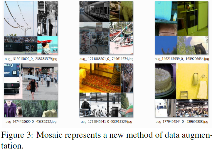
Mosaic represents a new data augmentation method that mixes 4 training images. Thus 4 different contexts are mixed, while CutMix mixes only 2 input images. This allows detection of objects outside their normal context. In addition, batch normalization calculates activation statistics from 4 different images on each layer. This significantly reduces the need for a large mini-batch size.

Mosaic 是一种新的数据增强方法，它将 4 幅训练图像混合在一起。这样就混合了 4 种不同的背景，而 CutMix 只混合了 2 幅输入图像。这样就可以检测到正常背景之外的目标。此外，批量归一化还能从每一层的 4 幅不同图像中计算激活统计数据。这大大降低了对大小批量的需求。

Self-Adversarial Training (SAT) also represents a new data augmentation technique that operates in 2 forward backward stages. In the 1st stage the neural network alters the original image instead of the network weights. In this way the neural network executes an adversarial attack on itself, altering the original image to create the deception that there is no desired object on the image. In the 2nd stage, the neural network is trained to detect an object on this modified image in the normal way.

Self-Adversarial Training(SAT)也是一种新的数据增强技术，它分为两个向前向后的阶段。在第一阶段，神经网络改变原始图像而不是网络权重。这样，神经网络就会对自己实施对抗性攻击，改变原始图像，制造图像上没有目标的假象。在第二阶段，对神经网络进行训练，使其能够以正常的方式检测修改后图像上的目标。

CmBN represents a CBN modified version, as shown in Figure 4, defined as Cross mini-Batch Normalization(CmBN). This collects statistics only between mini-batches within a single batch.

CmBN 是 CBN 的改进版，如图 4 所示，定义为跨小批量归一化（CmBN）。它只收集单个批次中迷你批次之间的统计数据。

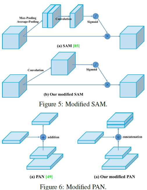
We modify SAM from spatial-wise attention to pointwise attention, and replace shortcut connection of PAN to concatenation, as shown in Figure 5 and Figure 6, respectively.

如图 5 和图 6 所示，我们将 SAM 从空间注意力修改为点注意力，并将 PAN 的快捷连接改为串联。

3.4 YOLOV4

In this section, we shall elaborate the details of YOLOv4.

YOLOv4 consists of:

• Backbone: CSPDarknet53 [81]
• Neck: SPP [25], PAN [49]
• Head: YOLOv3 [63]

YOLO v4 uses:

• Bag of Freebies (BoF) for backbone: CutMix and Mosaic data augmentation, DropBlock regularization, Class label smoothing
• Bag of Specials (BoS) for backbone: Mish activation, Cross-stage partial connections (CSP), Multiinput weighted residual connections (MiWRC)
• Bag of Freebies (BoF) for detector: CIoU-loss, CmBN, DropBlock regularization, Mosaic data augmentation, Self-Adversarial Training, Eliminate grid sensitivity, Using multiple anchors for a single ground truth, Cosine annealing scheduler [52], Optimal hyperparameters, Random training shapes
• Bag of Specials (BoS) for detector: Mish activation, SPP-block, SAM-block, PAN path-aggregation block, DIoU-NMS

在本节中，我们将详细阐述 YOLOv4 的细节。

YOLOv4 包括：

• 骨干网： CSPDarknet53 [81]
• 颈部 SPP [25], Pan [49]
• 头部：YOLOv3 [63]

YOLO v4 使用：

• 用于backbone的Bag of Freebies（BoF）： CutMix 和 Mosaic 数据增强、DropBlock 正则化、类标签平滑化
• 用于backbone的 Bag Of Specials (BoS)： Mish 激活、跨阶段部分连接 (CSP)、多输入加权残差连接 (MiWRC)
• 用于检测器的Bag of Freebies(BoF)： CIoU-loss, CmBN, DropBlock 正则化, Mosaic数据增强, 自我辩护训练, 消除网格敏感性, 使用多个锚点实现单一地面真实, 余弦退火调度器 [52], 最佳超参数, 随机训练形状
• 用于检测器的 Bag Of Specials (BoS)： Mish 激活、SPP 块、SAM 块、PAN 路径聚合块、DIoU-NMS

4 Experiments

We test the influence of different training improvement techniques on accuracy of the classifier on ImageNet (ILSVRC 2012 val) dataset, and then on the accuracy of the detector on MS COCO (test-dev 2017) dataset.

我们在 ImageNet（ILSVRC 2012 val）数据集上测试了不同训练改进技术对分类器准确性的影响，然后在 MS COCO（test-dev 2017）数据集上测试了检测器准确性的影响。

4.1. Experimental setup

In ImageNet image classification experiments, the default hyper-parameters are as follows: the training steps is 8,000,000; the batch size and the mini-batch size are 128 and 32, respectively; the polynomial decay learning rate scheduling strategy is adopted with initial learning rate 0.1; the warm-up steps is 1000; the momentum and weight decay are respectively set as 0.9 and 0.005. All of our BoS experiments use the same hyper-parameter as the default setting, and in the BoF experiments, we add an additional 50% training steps. In the BoF experiments, we verify MixUp, CutMix, Mosaic, Bluring data augmentation, and label smoothing regularization methods. In the BoS experiments, we compared the effects of LReLU, Swish, and Mish activation function. All experiments are trained with a 1080 Ti or 2080 Ti GPU.

在 ImageNet 图像分类实验中，默认的超参数如下：训练步数为 8,000,000；批量大小和小批量大小分别为 128 和 32；采用多项式衰减学习率调度策略，初始学习率为 0.1；预热步数为 1000；动量和权重衰减分别设置为 0.9 和 0.005。所有 BoS 实验都使用了与默认设置相同的超参数，而在 BoF 实验中，我们额外增加了 50%的训练步数。在 BoF 实验中，我们验证了 MixUp、CutMix、Mosaic、Bluring 数据增强和标签平滑正则化方法。在 BoS 实验中，我们比较了 LReLU、Swish 和 Mish 激活函数的效果。所有实验均使用 1080 Ti 或 2080 Ti GPU 进行训练。

In MS COCO object detection experiments, the default hyper-parameters are as follows: the training steps is 500,500; the step decay learning rate scheduling strategy is adopted with initial learning rate 0.01 and multiply with a factor 0.1 at the 400,000 steps and the 450,000 steps, respectively; The momentum and weight decay are respectively set as 0.9 and 0.0005. All architectures use a single GPU to execute multi-scale training in the batch size of 64 while mini-batch size is 8 or 4 depend on the architectures and GPU memory limitation. Except for using genetic algorithm for hyper-parameter search experiments, all other experiments use default setting. Genetic algorithm used YOLOv3-SPP to train with GIoU loss and search 300 epochs for min-val 5k sets. We adopt searched learning rate 0.00261, momentum 0.949, IoU threshold for assigning ground truth 0.213, and loss normalizer 0.07 for genetic algorithm experiments. We have verified a large number of BoF, including grid sensitivity elimination, mosaic data augmentation, IoU threshold, genetic algorithm, class label smoothing, cross mini-batch normalization, selfadversarial training, cosine annealing scheduler, dynamic mini-batch size, DropBlock, Optimized Anchors, different kind of IoU losses. We also conduct experiments on various BoS, including Mish, SPP, SAM, RFB, BiFPN, and Gaussian YOLO [8]. For all experiments, we only use one GPU for training, so techniques such as syncBN that optimizes multiple GPUs are not used.

在 MS COCO 目标检测实验中，默认超参数如下：训练步数为 500500 步；采用阶跃衰减学习率调度策略，初始学习率为 0.01，在 400000 步和 450000 步时分别乘以系数 0.1；动量和权重衰减分别设置为 0.9 和 0.0005。所有架构都使用单个 GPU 执行多尺度训练，批量为 64，而小批量为 8 或 4，这取决于架构和 GPU 内存限制。除了在超参数搜索实验中使用遗传算法外，其他实验均使用默认设置。遗传算法使用 YOLOv3-SPP 以 GIoU 损失进行训练，并对最小值 5k 集搜索 300 个历元。我们在遗传算法实验中采用了搜索学习率 0.00261、动量 0.949、分配 ground truth 的 IoU 阈值 0.213 和损失归一化 0.07。我们验证了大量 BoF，包括网格敏感度消除、马赛克数据增强、IoU 门限、遗传算法、类标签平滑、交叉小批量归一化、自对抗训练、余弦退火调度器、动态小批量、DropBlock、优化锚点、不同类型的 IoU 损失。我们还对各种 BoS 进行了实验，包括 Mish、SPP、SAM、RFB、BiFPN 和高斯 YOLO [8]。在所有实验中，我们只使用一个 GPU 进行训练，因此没有使用对多个 GPU 进行优化的 syncBN 等技术。

4.2 Influence of different features on Classifier training

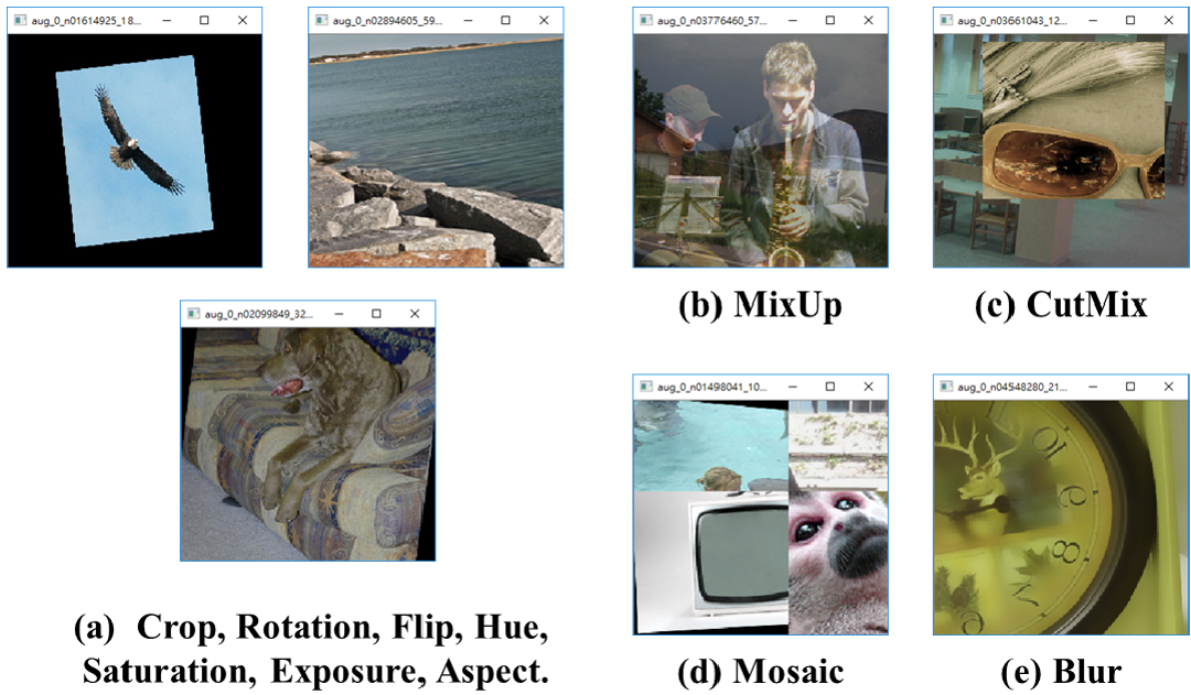
First, we study the influence of different features on classifier training; specifically, the influence of Class label smoothing, the influence of different data augmentation techniques, bilateral blurring, MixUp, CutMix and Mosaic, as shown in Fugure 7, and the influence of different activations, such as Leaky-ReLU (by default), Swish, and Mish.

首先，我们研究了不同特征对分类器训练的影响；具体来说，如图 7 所示，研究了类标签平滑的影响，不同数据增强技术、双边模糊、MixUp、CutMix 和 Mosaic 的影响，以及不同激活的影响，如 Leaky-ReLU（默认）、Swish 和 Mish。

Figure 7: Various method of data augmentation.

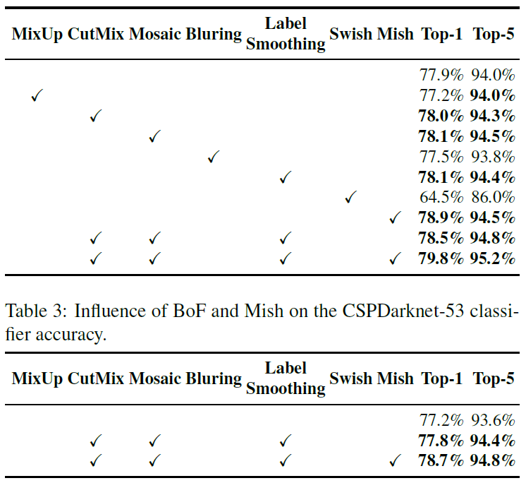
In our experiments, as illustrated in Table 2, the classifier’s accuracy is improved by introducing the features such as: CutMix and Mosaic data augmentation, Class label smoothing, and Mish activation. As a result, our BoFbackbone (Bag of Freebies) for classifier training includes the following: CutMix and Mosaic data augmentation and Class label smoothing. In addition we use Mish activation as a complementary option, as shown in Table 2 and Table 3.

在我们的实验中，如表 2 所示，通过引入 CutMix 和 Mosaic 数据增强、类标签平滑和 Mish 激活等特征，分类器的准确率得到了提高： CutMix 和 Mosaic 数据增强、类标签平滑和 Mish 激活。因此，我们用于分类器训练的 BoFbackbone（Bag of Freebies）包括以下内容： CutMix 和 Mosaic 数据增强以及类标签平滑。此外，我们还使用 Mish 激活作为补充选项，如表 2 和表 3 所示。

4.3. Influence of different features on Detector training

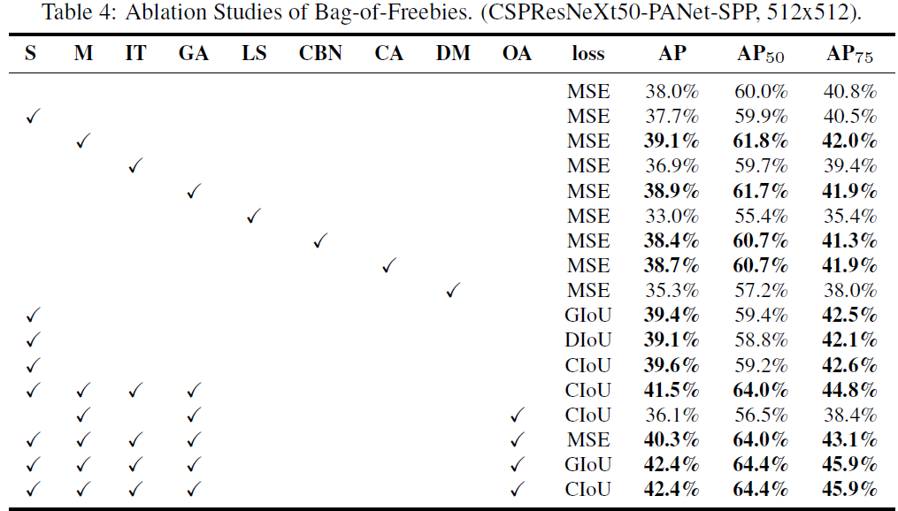
Further study concerns the influence of different Bag-of-Freebies (BoF-detector) on the detector training accuracy, as shown in Table 4. We significantly expand the BoF list through studying different features that increase the detector accuracy without affecting FPS:

如表 4 所示，进一步的研究涉及不同的 “big of freebies”（BoF-detector）对检测器训练精度的影响。我们通过研究在不影响 FPS 的情况下提高检测器精度的不同特征，大大扩展了 BoF 列表：

• S: Eliminate grid sensitivity the equation $b_x=\sigma (tx)+c_x$; $b_y=\sigma (t_y)+c_y$, where $c_x$ and $c_y$ are always whole numbers, is used in YOLOv3 for evaluating the object coordinates, therefore, extremely high $t_x$ absolute values are required for the bx value approaching the $c_x$ or $c_x+1$ values. We solve this problem through multiplying the sigmoid by a factor exceeding 1.0, so eliminating the effect of grid on which the object is undetectable.

  S：消除网格灵敏度 YOLOv3 中使用方程 $b_x=\sigma (tx)+c_x$；$b_y=\sigma (t_y)+c_y$，其中 $c_x$ 和 $c_y$ 始终为整数，用于评估物体坐标，因此需要极高的 $t_x$ 绝对值才能使 $b_x$ 值接近 $c_x$ 或 $c_x+1$。我们通过将 sigmoid 乘以一个超过 1.0 的系数来解决这个问题，从而消除了无法探测到物体的网格的影响。

• M: Mosaic data augmentation — using the 4-image mosaic during training instead of single image

  M：马赛克数据增强–在训练过程中使用 4 幅马赛克图像，而不是单幅图像

• IT: IoU threshold - using multiple anchors for a single ground truth IoU (truth, anchor) > IoU_threshold

  IT：IoU阈值–使用多个锚点来获取单一地面实况 IoU（真相，锚点）> IoU_阈值

• GA: Genetic algorithms - using genetic algorithms for selecting the optimal hyperparameters during network training on the first 10% of time periods

  GA： 遗传算法 遗传算法–在网络训练过程中，使用遗传算法在前 10%的时间段内选择最佳超参数

• LS: Class label smoothing - using class label smoothing for sigmoid activation

  LS：类标签平滑法–使用类标签平滑法进行 sigmoid 激活

• CBN: CmBN - using Cross mini-Batch Normalization for collecting statistics inside the entire batch, instead of collecting statistics inside a single mini-batch

  CBN： CmBN：交叉迷你批归一化–使用交叉迷你批归一化收集整个批次的统计数据，而不是收集单个迷你批次的统计数据

• CA: Cosine annealing scheduler - altering the learning rate during sinusoid training

  CA：余弦退火调度器–在正弦训练过程中改变学习率

• DM: Dynamic mini-batch size - automatic increase of mini-batch size during small resolution training by using Random training shapes

  DM：动态小批量–通过使用随机训练形状，在小分辨率训练期间自动增加小批量规模

• OA: Optimized Anchors - using the optimized anchors for training with the 512x512 network resolution GIoU, CIoU, DIoU, MSE - using different loss algorithms for bounded box regression

  OA：优化锚点–使用优化锚点进行 512x512 网络分辨率训练 GIoU、CIoU、DIoU、MSE–使用不同损失算法进行有界箱回归

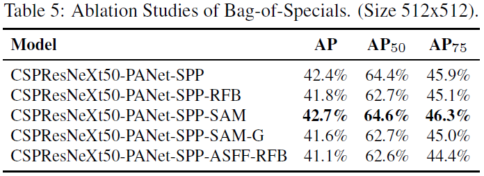
Further study concerns the influence of different Bagof-Specials (BoS-detector) on the detector training accuracy, including PAN, RFB, SAM, Gaussian YOLO (G), and ASFF, as shown in Table 5. In our experiments, the detector gets best performance when using SPP, PAN, and SAM.

如表 5 所示，进一步的研究涉及不同特征包（BoS-检测器）对检测器训练精度的影响，包括 PAN、RFB、SAM、高斯 YOLO (G) 和 ASFF。在我们的实验中，检测器在使用 SPP、PAN 和 SAM 时性能最佳。

4.4. Influence of different backbones and pretrained weightings on Detector training

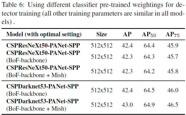
Further on we study the influence of different backbone models on the detector accuracy, as shown in Table 6. We notice that the model characterized with the best classification accuracy is not always the best in terms of the detector accuracy.

如表 6 所示，我们进一步研究了不同骨干网模型对检测器精度的影响。我们注意到，分类准确率最高的模型并不总是检测器准确率最高的模型。

First, although classification accuracy of CSPResNeXt-50 models trained with different features is higher compared to CSPDarknet53 models, the CSPDarknet53 model shows higher accuracy in terms of object detection.

首先，虽然与 CSPDarknet53 模型相比，使用不同特征训练的 CSPResNeXt-50 模型的分类准确率更高，但在目标检测方面，CSPDarknet53 模型显示出更高的准确率。

Second, using BoF and Mish for the CSPResNeXt50 classifier training increases its classification accuracy, but further application of these pre-trained weightings for detector training reduces the detector accuracy. However, using BoF and Mish for the CSPDarknet53 classifier training increases the accuracy of both the classifier and the detector which uses this classifier pre-trained weightings. The net result is that backbone CSPDarknet53 is more suitable for the detector than for CSPResNeXt50.

其次，在 CSPResNeXt50 分类器训练中使用 BoF 和 Mish 可以提高分类器的分类准确率，但在检测器训练中进一步使用这些预训练加权则会降低检测器的准确率。然而，在 CSPDarknet53 分类器训练中使用 BoF 和 Mish 会提高分类器和使用该分类器预训练加权的检测器的准确性。最终结果是，骨干 CSPDarknet53 比 CSPResNeXt50 更适合检测器。

We observe that the CSPDarknet53 model demonstrates a greater ability to increase the detector accuracy owing to various improvements.

我们注意到，由于各种改进，CSPDarknet53 模型在提高检测器准确性方面表现出更强的能力。

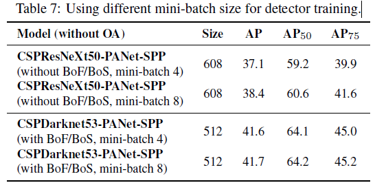
4.5. Influence of different minibatch size on Detector training

Finally, we analyze the results obtained with models trained with different mini-batch sizes, and the results are shown in Table 7. From the results shown in Table 7, we found that after adding BoF and BoS training strategies, the mini-batch size has almost no effect on the detector’s performance. This result shows that after the introduction of BoF and BoS, it is no longer necessary to use expensive GPUs for training. In other words, anyone can use only a conventional GPU to train an excellent detector.

最后，我们分析了用不同小批量训练的模型得到的结果，结果如表 7 所示。从表 7 所示的结果中，我们发现在加入 BoF 和 BoS 训练策略后，小批量对检测器的性能几乎没有影响。这一结果表明，引入 BoF 和 BoS 后，不再需要使用昂贵的 GPU 进行训练。换句话说，任何人只需使用传统的 GPU 就能训练出优秀的探测器。

5 Results

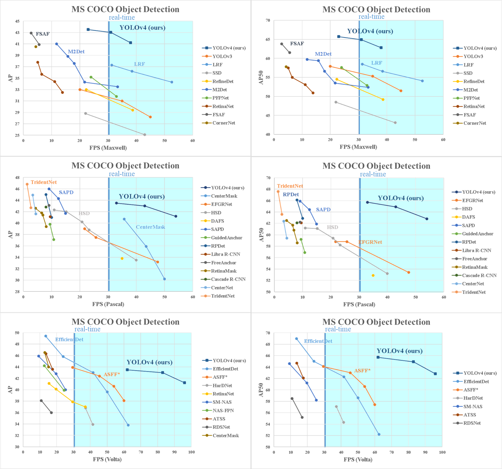
Comparison of the results obtained with other stateof-the-art object detectors are shown in Figure 8. Our YOLOv4 are located on the Pareto optimality curve and are superior to the fastest and most accurate detectors in terms of both speed and accuracy.

与其他最先进的目标检测器的比较结果如图 8 所示。我们的 YOLOv4 位于帕累托最优曲线上，在速度和精度方面都优于最快和最精确的检测器。

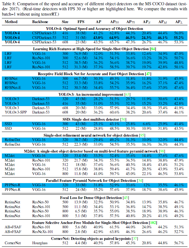
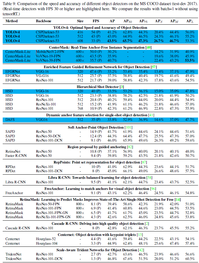
Since different methods use GPUs of different architectures for inference time verification, we operate YOLOv4 on commonly adopted GPUs of Maxwell, Pascal, and Volta architectures, and compare them with other state-of-the-art methods. Table 8 lists the frame rate comparison results of using Maxwell GPU, and it can be GTX Titan X (Maxwell) or Tesla M40 GPU. Table 9 lists the frame rate comparison results of using Pascal GPU, and it can be Titan X (Pascal), Titan Xp, GTX 1080 Ti, or Tesla P100 GPU. As for Table 10, it lists the frame rate comparison results of using Volta GPU, and it can be Titan Volta or Tesla V100 GPU.

由于不同的方法使用不同架构的 GPU 进行推理时间验证，我们在常用的 Maxwell、Pascal 和 Volta 架构 GPU 上运行 YOLOv4，并与其他最先进的方法进行比较。表 8 列出了使用 Maxwell GPU（可以是 GTX Titan X（Maxwell）或 Tesla M40 GPU）的帧速率比较结果。表 9 列出了使用 Pascal GPU 的帧速率对比结果，可以是 Titan X（Pascal）、Titan Xp、GTX 1080 Ti 或 Tesla P100 GPU。表 10 列出了使用 Volta GPU 的帧速率对比结果，可以是 Titan Volta 或 Tesla V100 GPU。

Figure 8: Comparison of the speed and accuracy of different object detectors. (Some articles stated the FPS of their detectors for only one of the GPUs: Maxwell/Pascal/Volta)

6 Conclusions

We offer a state-of-the-art detector which is faster (FPS) and more accurate (MS COCO AP50…95 and AP50) than all available alternative detectors. The detector described can be trained and used on a conventional GPU with 8-16 GB-VRAM this makes its broad use possible. The original concept of one-stage anchor-based detectors has proven its viability. We have verified a large number of features, and selected for use such of them for improving the accuracy of both the classifier and the detector. These features can be used as best-practice for future studies and developments.

我们提供了一种最先进的检测器，它比现有的所有检测器都更快（FPS）、更准确（MS COCO AP50…95 和 AP50）。所述检测器可在配备 8-16 GB-VRAM 的传统 GPU 上进行训练和使用，这使其广泛应用成为可能。基于锚点的单级检测器的原始概念已经证明了其可行性。我们验证了大量特征，并选择了其中一些特征用于提高分类器和检测器的准确性。这些特征可作为未来研究和开发的最佳实践。

7 Acknowledgements

The authors wish to thank Glenn Jocher for the ideas of Mosaic data augmentation, the selection of hyper-parameters by using genetic algorithms and solving the grid sensitivity problem https://github.com/ultralytics/yolov3.

作者感谢 Glenn Jocher 提出的 Mosaic 数据扩增、使用遗传算法选择超参数和解决网格敏感性问题的想法 https://github.com/ultralytics/yolov3。