CS231n课程学习笔记（二）——SVM的实现

最新推荐文章于 2024-07-11 18:30:49 发布

StarCoo

最新推荐文章于 2024-07-11 18:30:49 发布

阅读量2.5k

点赞数 4

分类专栏：深度学习文章标签： svm

本文链接：https://blog.csdn.net/stalbo/article/details/79379070

版权

深度学习专栏收录该内容

10 篇文章 6 订阅

订阅专栏

翻译笔记：https://zhuanlan.zhihu.com/p/21930884?refer=intelligentunit
作业讲解视频地址：http://www.mooc.ai/course/364/learn#lesson/2118

作业讲解

求损失Loss

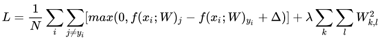
多分类线性SVM： $y=Wx$
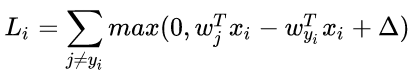
Hinge Loss（Max margin），margin=1：

注意：这个式子中只有错误的分类才会产生loss，即j=i 正确分类是没有loss的。
设置Delta：超参数 $\Delta$ 应该被设置成什么值？需要通过交叉验证来求得吗？在绝大多数情况下该超参数设为 $\Delta=1.0$ 都是安全的。

实现代码如下：

scores=X.dot(W)
margin=scores-scores[np.arange(num_train),y].reshape(num_train,1)+1
margin[np.arange(num_train),y]=0.0#正确的这一列不该计算，归零
margin=(margin>0)*margin
loss+=margin.sum()/num_train
loss+=0.5*reg*np.sum(W*W)#乘0.5，因为后面是平方，求导时有一个2可以与0.5相乘为1

求梯度dW

Loss计算公式：
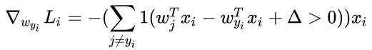
梯度：

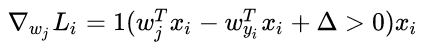
其中 $1$ 是一个示性函数，如果括号中的条件为真，那么函数值为 $1$ ，如果为假，则函数值为 $0$ 。虽然上述公式看起来复杂，但在代码实现的时候比较简单：只需要计算没有满足边界值的分类的数量（因此对损失函数产生了贡献），然后乘以 $x_{i}$ 就是梯度了。注意，这个梯度只是对应正确分类的 $W$ 的行向量的梯度，那些 $j\not =y_{i}$ 行的梯度是：

具体实现代码：

margin=(margin>0)*1
row_sum=np.sum(margin,axis=1)
margin[np.arange(num_train),y]=-row_sum
dW=X.T.dot(margin)/num_train+reg*W

总体代码展示

打开svm.ipynb：

import random
import numpy as np
from cs231n.data_utils import load_CIFAR10
import matplotlib.pyplot as plt

plt.rcParams['figure.figsize'] = (10.0, 8.0) # set default size of plots
plt.rcParams['image.interpolation'] = 'nearest'
plt.rcParams['image.cmap'] = 'gray'

数据加载和预处理

与之前KNN相同，加载数据后可以显示一部分样本

# Load the raw CIFAR-10 data.
cifar10_dir = 'cs231n/datasets/cifar-10-batches-py'
X_train, y_train, X_test, y_test = load_CIFAR10(cifar10_dir)

classes = ['plane', 'car', 'bird', 'cat', 'deer', 'dog', 'frog', 'horse', 'ship', 'truck']
num_classes = len(classes)
samples_per_class = 7
for y, cls in enumerate(classes):
    idxs = np.flatnonzero(y_train == y)
    idxs = np.random.choice(idxs, samples_per_class, replace=False)
    for i, idx in enumerate(idxs):
        plt_idx = i * num_classes + y + 1
        plt.subplot(samples_per_class, num_classes, plt_idx)
        plt.imshow(X_train[idx].astype('uint8'))
        plt.axis('off')
        if i == 0:
            plt.title(cls)
plt.show()

将数据集分为训练集、交叉验证集和测试集，并从训练集中分出一个小的子集

num_training = 49000
num_validation = 1000
num_test = 1000
num_dev = 500

mask = range(num_training, num_training + num_validation)
X_val = X_train[mask]
y_val = y_train[mask]

mask = range(num_training)
X_train = X_train[mask]
y_train = y_train[mask]

# We will also make a development set, which is a small subset of
# the training set.
mask = np.random.choice(num_training, num_dev, replace=False)
X_dev = X_train[mask]
y_dev = y_train[mask]

# We use the first num_test points of the original test set as our
# test set.
mask = range(num_test)
X_test = X_test[mask]
y_test = y_test[mask]

print ('Train data shape: ', X_train.shape)
print ('Train labels shape: ', y_train.shape)
print ('Validation data shape: ', X_val.shape)
print ('Validation labels shape: ', y_val.shape)
print ('Test data shape: ', X_test.shape)
print ('Test labels shape: ', y_test.shape)

OUTPUT：
Train data shape: (49000, 32, 32, 3)
Train labels shape: (49000,)
Validation data shape: (1000, 32, 32, 3)
Validation labels shape: (1000,)
Test data shape: (1000, 32, 32, 3)
Test labels shape: (1000,)

改变数据维度，将每一张图片用一行向量来表示：

# Preprocessing: reshape the image data into rows
X_train = np.reshape(X_train, (X_train.shape[0], -1))
X_val = np.reshape(X_val, (X_val.shape[0], -1))
X_test = np.reshape(X_test, (X_test.shape[0], -1))
X_dev = np.reshape(X_dev, (X_dev.shape[0], -1))

# As a sanity check, print out the shapes of the data
print ('Training data shape: ', X_train.shape)
print ('Validation data shape: ', X_val.shape)
print ('Test data shape: ', X_test.shape)
print ('dev data shape: ', X_dev.shape)

OUTPUT：
Training data shape: (49000, 3072)
Validation data shape: (1000, 3072)
Test data shape: (1000, 3072)
dev data shape: (500, 3072)

Normalize data 基于训练集，算出图片的均值，并减去。

mean_image = np.mean(X_train, axis=0)
X_train -= mean_image
X_val -= mean_image
X_test -= mean_image
X_dev -= mean_image

数据矩阵加上偏差列，方便之后的计算

X_train = np.hstack([X_train, np.ones((X_train.shape[0], 1))])
X_val = np.hstack([X_val, np.ones((X_val.shape[0], 1))])
X_test = np.hstack([X_test, np.ones((X_test.shape[0], 1))])
X_dev = np.hstack([X_dev, np.ones((X_dev.shape[0], 1))])

print (X_train.shape, X_val.shape, X_test.shape, X_dev.shape)

OUTPUT：
(49000, 3073) (1000, 3073) (1000, 3073) (500, 3073)

SVM分类器的实现

打开cs231n\classifiers文件夹中的 linear_svm.py 完成SVM的实现代码。

损失函数和梯度

方法一：

def svm_loss_naive(W, X, y, reg):

  dW = np.zeros(W.shape) # initialize the gradient as zero

  # compute the loss and the gradient
  num_classes = W.shape[1]
  num_train = X.shape[0]
  loss = 0.0
  for i in range(num_train):
      scores = X[i].dot(W)
      correct_class_score = scores[y[i]]
      for j in range(num_classes):
          if j == y[i]:
              continue
          margin = scores[j] - correct_class_score + 1# delta=1
          if margin > 0:#max(0,--)操作
              loss += margin
              dW[:,y[i]] += -X[i] #对应正确分类的梯度 (D,)
              dW[:,j] += X[i] #对应不正确分类的梯度

  # Right now the loss is a sum over all training examples, but we want it
  # to be an average instead so we divide by num_train.
  loss /= num_train
  dW/=num_train
  # Add regularization to the loss.
  loss += 0.5 * reg * np.sum(W * W)
  dW += reg*W

  return loss, dW

方法二矢量化版：

def svm_loss_vectorized(W, X, y, reg):

  loss = 0.0
  dW = np.zeros(W.shape) # initialize the gradient as zero

  num_train = X.shape[0]

  scores = X.dot(W)
  margin = scores-scores[np.arange(num_train),y].reshape(num_train,1)+1
  margin[np.arange(num_train),y] = 0.0#正确的这一列不该计算，归零
  margin = (margin > 0)*margin
  loss += margin.sum()/num_train
  loss += 0.5*reg*np.sum(W*W)

  margin = (margin > 0)*1
  row_sum = np.sum(margin,axis=1)
  margin[np.arange(num_train),y] = -row_sum
  dW = X.T.dot(margin)/num_train + reg*W


  return loss, dW

梯度检查

返回svm.ipynb：

loss, grad = svm_loss_naive(W, X_dev, y_dev, 0.0)

from cs231n.gradient_check import grad_check_sparse
f = lambda w: svm_loss_naive(w, X_dev, y_dev, 0.0)[0]
grad_numerical = grad_check_sparse(f, W, grad)

loss, grad = svm_loss_naive(W, X_dev, y_dev, 1e2)
f = lambda w: svm_loss_naive(w, X_dev, y_dev, 1e2)[0]
grad_numerical = grad_check_sparse(f, W, grad)

OUTPUT：
numerical: -7.714121 analytic: -7.714121, relative error: 2.882459e-11
numerical: 6.498201 analytic: 6.498201, relative error: 1.616181e-11
numerical: -5.996422 analytic: -5.996422, relative error: 2.548793e-11
numerical: 18.051604 analytic: 18.051604, relative error: 2.654182e-11
numerical: -5.968500 analytic: -5.968500, relative error: 1.546593e-12
numerical: -9.307208 analytic: -9.307208, relative error: 3.240868e-11
numerical: 1.955191 analytic: 1.955191, relative error: 8.351098e-11
numerical: -1.443719 analytic: -1.443719, relative error: 2.464525e-10
numerical: 8.680369 analytic: 8.680369, relative error: 5.149589e-11
numerical: 3.160608 analytic: 3.160608, relative error: 9.645160e-11
numerical: 3.229153 analytic: 3.229153, relative error: 6.157453e-11
numerical: 19.706387 analytic: 19.706387, relative error: 1.384803e-11
numerical: 4.034088 analytic: 4.034088, relative error: 4.787692e-11
numerical: -12.270168 analytic: -12.270168, relative error: 1.866756e-11
numerical: -2.268660 analytic: -2.268660, relative error: 3.041155e-11
numerical: -0.057320 analytic: -0.057320, relative error: 6.521383e-09
numerical: -7.380878 analytic: -7.380878, relative error: 3.713221e-11
numerical: 11.643386 analytic: 11.643386, relative error: 4.090276e-11
numerical: 15.993779 analytic: 15.993779, relative error: 7.325546e-12
numerical: -4.908855 analytic: -4.908855, relative error: 7.685458e-11

其中，梯度检查函数为：

def grad_check_sparse(f, x, analytic_grad, num_checks=10, h=1e-5):
  """
  sample a few random elements and only return numerical
  in this dimensions.
  """

  for i in range(num_checks):
    ix = tuple([randrange(m) for m in x.shape])

    oldval = x[ix]
    x[ix] = oldval + h # increment by h
    fxph = f(x) # evaluate f(x + h)
    x[ix] = oldval - h # increment by h
    fxmh = f(x) # evaluate f(x - h)
    x[ix] = oldval # reset

    grad_numerical = (fxph - fxmh) / (2 * h)
    grad_analytic = analytic_grad[ix]
    rel_error = abs(grad_numerical - grad_analytic) / (abs(grad_numerical) + abs(grad_analytic))
    print ('numerical: %f analytic: %f, relative error: %e' % (grad_numerical, grad_analytic, rel_error))

计算Loss和梯度

tic = time.time()
loss_naive, grad_naive = svm_loss_naive(W, X_dev, y_dev, 0.00001)
toc = time.time()
print ('Naive loss: %e computed in %fs' % (loss_naive, toc - tic))

from cs231n.classifiers.linear_svm import svm_loss_vectorized
tic = time.time()
loss_vectorized, _ = svm_loss_vectorized(W, X_dev, y_dev, 0.00001)
toc = time.time()
print ('Vectorized loss: %e computed in %fs' % (loss_vectorized, toc - tic))

# The losses should match but your vectorized implementation should be much faster.
print ('difference: %f' % (loss_naive - loss_vectorized))

OUTPUT：
Naive loss: 9.169259e+00 computed in 0.243172s
Vectorized loss: 9.169259e+00 computed in 0.127999s
difference: -0.000000

tic = time.time()
_, grad_naive = svm_loss_naive(W, X_dev, y_dev, 0.00001)
toc = time.time()
print ('Naive loss and gradient: computed in %fs' % (toc - tic))

tic = time.time()
_, grad_vectorized = svm_loss_vectorized(W, X_dev, y_dev, 0.00001)
toc = time.time()
print ('Vectorized loss and gradient: computed in %fs' % (toc - tic))

# The loss is a single number, so it is easy to compare the values computed
# by the two implementations. The gradient on the other hand is a matrix, so
# we use the Frobenius norm to compare them.
difference = np.linalg.norm(grad_naive - grad_vectorized, ord='fro')
print ('difference: %f' % difference)

OUTPUT：
Naive loss and gradient: computed in 0.279197s
Vectorized loss and gradient: computed in 0.008006s
difference: 0.000000

随机梯度下降

在linear_classifier.py 文件中实现SGD函数

更新权值和loss

 def train(self, X, y, learning_rate=1e-3, reg=1e-5, num_iters=100,
            batch_size=200, verbose=False):
    """
    Train this linear classifier using stochastic gradient descent.

    Inputs:
    - X: A numpy array of shape (N, D) containing training data; there are N
      training samples each of dimension D.
    - y: A numpy array of shape (N,) containing training labels; y[i] = c
      means that X[i] has label 0 <= c < C for C classes.
    - learning_rate: (float) learning rate for optimization.
    - reg: (float) regularization strength.
    - num_iters: (integer) number of steps to take when optimizing
    - batch_size: (integer) number of training examples to use at each step.
    - verbose: (boolean) If true, print progress during optimization.

    Outputs:
    A list containing the value of the loss function at each training iteration.
    """
    num_train, dim = X.shape
    num_classes = np.max(y) + 1 # assume y takes values 0...K-1 where K is number of classes
    if self.W is None:
      # lazily initialize W
      self.W = 0.001 * np.random.randn(dim, num_classes)

    # Run stochastic gradient descent to optimize W
    loss_history = []
    for it in range(num_iters):
      X_batch = None
      y_batch = None

      #########################################################################
      # TODO:                                                                 #
      # Sample batch_size elements from the training data and their           #
      # corresponding labels to use in this round of gradient descent.        #
      # Store the data in X_batch and their corresponding labels in           #
      # y_batch; after sampling X_batch should have shape (dim, batch_size)   #
      # and y_batch should have shape (batch_size,)                           #
      #                                                                       #
      # Hint: Use np.random.choice to generate indices. Sampling with         #
      # replacement is faster than sampling without replacement.              #
      #########################################################################
      #子采样
      mask = np.random.choice(num_train,batch_size,replace = False)#replace = False 没有重复
      X_batch = X[mask]
      y_batch = y[mask]
      #########################################################################
      #                       END OF YOUR CODE                                #
      #########################################################################

      # evaluate loss and gradient
      loss, grad = self.loss(X_batch, y_batch, reg)
      loss_history.append(loss)

      # perform parameter update
      #########################################################################
      # TODO:                                                                 #
      # Update the weights using the gradient and the learning rate.          #
      #########################################################################
      #梯度更新
      self.W += -learning_rate * grad
      #########################################################################
      #                       END OF YOUR CODE                                #
      #########################################################################

      if verbose and it % 100 == 0:
        print('iteration %d / %d: loss %f' % (it, num_iters, loss))

    return loss_history

返回svm.ipynb：

from cs231n.classifiers import LinearSVM
svm = LinearSVM()
tic = time.time()
loss_hist = svm.train(X_train, y_train, learning_rate=1e-7, reg=5e4,
                      num_iters=1500, verbose=True)
toc = time.time()
print ('That took %fs' % (toc - tic))

OUTPUT：
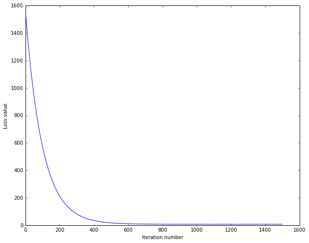
iteration 0 / 1500: loss 783.675906
iteration 100 / 1500: loss 286.361632
iteration 200 / 1500: loss 107.706003
iteration 300 / 1500: loss 42.079802
iteration 400 / 1500: loss 18.928470
iteration 500 / 1500: loss 10.308477
iteration 600 / 1500: loss 7.065352
iteration 700 / 1500: loss 6.034884
iteration 800 / 1500: loss 5.524071
iteration 900 / 1500: loss 5.358315
iteration 1000 / 1500: loss 5.227159
iteration 1100 / 1500: loss 5.353792
iteration 1200 / 1500: loss 4.651034
iteration 1300 / 1500: loss 5.133628
iteration 1400 / 1500: loss 5.408001
That took 16.869082s

# A useful debugging strategy is to plot the loss as a function of
# iteration number:
plt.plot(loss_hist)
plt.xlabel('Iteration number')
plt.ylabel('Loss value')
plt.show()

OUTPUT：

预测准确度

在linear_classifier.py 文件中实现predict函数

  def predict(self, X):
    """
    Use the trained weights of this linear classifier to predict labels for
    data points.

    Inputs:
    - X: D x N array of training data. Each column is a D-dimensional point.

    Returns:
    - y_pred: Predicted labels for the data in X. y_pred is a 1-dimensional
      array of length N, and each element is an integer giving the predicted
      class.
    """
    y_pred = np.zeros(X.shape[1])
    ###########################################################################
    # TODO:                                                                   #
    # Implement this method. Store the predicted labels in y_pred.            #
    ###########################################################################
    score = X.dot(self.W)
    index = np.zeros(X.shape[0])
    index = np.argmax(score,axis = 1)
    y_pred = index
    ###########################################################################
    #                           END OF YOUR CODE                              #
    ###########################################################################
    return y_pred

得到预测label后，计算精度：

# Write the LinearSVM.predict function and evaluate the performance on both the
# training and validation set
y_train_pred = svm.predict(X_train)
print ('training accuracy: %f' % (np.mean(y_train == y_train_pred), ))
y_val_pred = svm.predict(X_val)
print ('validation accuracy: %f' % (np.mean(y_val == y_val_pred), ))

利用交叉验证集调整超参数

# Use the validation set to tune hyperparameters (regularization strength and
# learning rate). You should experiment with different ranges for the learning
# rates and regularization strengths; if you are careful you should be able to
# get a classification accuracy of about 0.4 on the validation set.
learning_rates = [1e-7, 5e-5]
regularization_strengths = [5e4, 1e5]

# results is dictionary mapping tuples of the form
# (learning_rate, regularization_strength) to tuples of the form
# (training_accuracy, validation_accuracy). The accuracy is simply the fraction
# of data points that are correctly classified.
results = {}
best_val = -1   # The highest validation accuracy that we have seen so far.
best_svm = None # The LinearSVM object that achieved the highest validation rate.

################################################################################
# TODO:                                                                        #
# Write code that chooses the best hyperparameters by tuning on the validation #
# set. For each combination of hyperparameters, train a linear SVM on the      #
# training set, compute its accuracy on the training and validation sets, and  #
# store these numbers in the results dictionary. In addition, store the best   #
# validation accuracy in best_val and the LinearSVM object that achieves this  #
# accuracy in best_svm.                                                        #
#                                                                              #
# Hint: You should use a small value for num_iters as you develop your         #
# validation code so that the SVMs don't take much time to train; once you are #
# confident that your validation code works, you should rerun the validation   #
# code with a larger value for num_iters.                                      #
################################################################################
iters = 2000 #100
for lr in learning_rates:
    for rs in regularization_strengths:
        svm = LinearSVM()
        svm.train(X_train, y_train, learning_rate=lr, reg=rs, num_iters=iters)

        y_train_pred = svm.predict(X_train)
        acc_train = np.mean(y_train == y_train_pred)
        y_val_pred = svm.predict(X_val)
        acc_val = np.mean(y_val == y_val_pred)

        results[(lr, rs)] = (acc_train, acc_val)

        if best_val < acc_val:
            best_val = acc_val
            best_svm = svm
################################################################################
#                              END OF YOUR CODE                                #
################################################################################

# Print out results.
for lr, reg in sorted(results):
    train_accuracy, val_accuracy = results[(lr, reg)]
    print ('lr %e reg %e train accuracy: %f val accuracy: %f' % (
                lr, reg, train_accuracy, val_accuracy))

print ('best validation accuracy achieved during cross-validation: %f' % best_val)

OUTPUT：
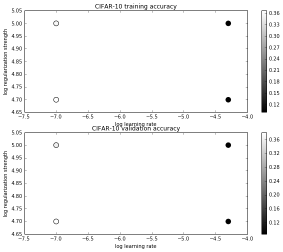
lr 1.000000e-07 reg 5.000000e+04 train accuracy: 0.370633 val accuracy: 0.379000
lr 1.000000e-07 reg 1.000000e+05 train accuracy: 0.358286 val accuracy: 0.366000
lr 5.000000e-05 reg 5.000000e+04 train accuracy: 0.100265 val accuracy: 0.087000
lr 5.000000e-05 reg 1.000000e+05 train accuracy: 0.100265 val accuracy: 0.087000
best validation accuracy achieved during cross-validation: 0.379000

可视化结果：

# Visualize the cross-validation results
import math
x_scatter = [math.log10(x[0]) for x in results]
y_scatter = [math.log10(x[1]) for x in results]

# plot training accuracy
marker_size = 100
colors = [results[x][0] for x in results]
plt.subplot(2, 1, 1)
plt.scatter(x_scatter, y_scatter, marker_size, c=colors)
plt.colorbar()
plt.xlabel('log learning rate')
plt.ylabel('log regularization strength')
plt.title('CIFAR-10 training accuracy')

# plot validation accuracy
colors = [results[x][1] for x in results] # default size of markers is 20
plt.subplot(2, 1, 2)
plt.scatter(x_scatter, y_scatter, marker_size, c=colors)
plt.colorbar()
plt.xlabel('log learning rate')
plt.ylabel('log regularization strength')
plt.title('CIFAR-10 validation accuracy')
plt.show()

OUTPUT：

在测试集上验证

# Evaluate the best svm on test set
y_test_pred = best_svm.predict(X_test)
test_accuracy = np.mean(y_test == y_test_pred)
print ('linear SVM on raw pixels final test set accuracy: %f' % test_accuracy)

OUTPUT： linear SVM on raw pixels final test set accuracy: 0.370000

# Visualize the learned weights for each class.
# Depending on your choice of learning rate and regularization strength, these may
# or may not be nice to look at.
w = best_svm.W[:-1,:] # strip out the bias
w = w.reshape(32, 32, 3, 10)
w_min, w_max = np.min(w), np.max(w)
classes = ['plane', 'car', 'bird', 'cat', 'deer', 'dog', 'frog', 'horse', 'ship', 'truck']
for i in range(10):
  plt.subplot(2, 5, i + 1)

  # Rescale the weights to be between 0 and 255
  wimg = 255.0 * (w[:, :, :, i].squeeze() - w_min) / (w_max - w_min)
  plt.imshow(wimg.astype('uint8'))
  plt.axis('off')
  plt.title(classes[i])

OUTPUT：

StarCoo

关注

4
点赞
踩
17

收藏

觉得还不错? 一键收藏
0
评论
CS231n课程学习笔记（二）——SVM的实现

翻译笔记：https://zhuanlan.zhihu.com/p/21930884?refer=intelligentunit 作业讲解视频地址：http://www.mooc.ai/course/364/learn#lesson/2118作业讲解求损失Loss多分类线性SVM：y=Wxy=Wxy=WxHinge Loss（Max margin），margin=1： ...
复制链接

扫一扫

专栏目录