


0. 引子
自从半年前开始进入418实验室研究深度学习,可以说caffe这一深度学习开源框架,一直伴随着我。经过了大半年的学习,虽然还有许多东西尚待完善,但起码对于caffe已经有了一个比较感性的认识。互联网上,关于深度学习和caffe的资料汗牛充栋,但质量往往参差不齐。我搜集了一些资料,加入自己的理解,总结在这里,也是对自己的一个督促吧。
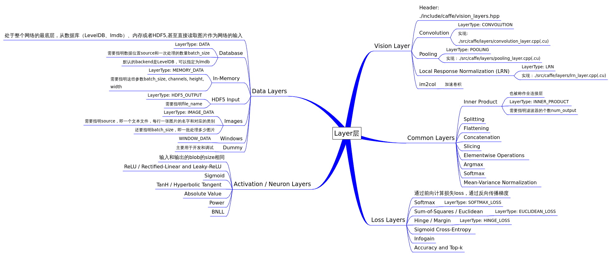
本文主要总结了caffe框架中的各种layer。layer是神经网络搭建的脚手架,理解了layer,才能更好地理解NN(Neural Networks)。
下面这张图是我在网络上搜集的一张关于layer的思维导图,我觉得总结的挺好。有心人可以看完全文后,再回过头来看这张图,相信一定会有新的理解。
1. Outline
这个Section主要概述了与layer有关的方方面面。
1.1. layer.hpp
和layer相关的头文件有:
layer.hpp

common_layers.hpp
data_layers.hpp
loss_layers.hpp
neuron_layers.hpp
vision_layers.hpp
其中layer.hpp是抽象出来的基类,其他都是在其基础上的继承,也即剩下的五个头文件和上图中的五个部分。在layer.hpp头文件里,包含了这几个头文件:
#include "caffe/blob.hpp"
#include "caffe/common.hpp"
#include "caffe/proto/caffe.pb.h"
#include "caffe/util/device_alternate.hpp"
在device_alternate.hpp中,通过#ifdef CPU_ONLY定义了一些宏来取消GPU的调用:
#define STUB_GPU(classname)
#define STUB_GPU_FORWARD(classname, funcname)
#define STUB_GPU_BACKWARD(classname, funcname)
layer中有这三个主要参数:
LayerParameter layer_param_;           // 这个是protobuf文件中存储的layer参数
vector<share_ptr<Blob<Dtype>>> blobs_; // 这个存储的是layer的参数,在程序中用的
vector<bool> param_propagate_down_;    // 这个bool表示是否计算各个blob参数的diff,即传播误差
Layer类的构建函数 explicit Layer(const LayerParameter& param) : layer_param_(param) 会尝试从protobuf文件读取参数。其三个主要接口:
virtual void SetUp(const vector<Blob<Dtype>*>& bottom, vector<Blob<Dtype>*>* top)
inline Dtype Forward(const vector<Blob<Dtype>*>& bottom, vector<Blob<Dtype>*>* top);
inline void Backward(const vector<Blob<Dtype>*>& top, const vector<bool>& propagate_down, const <Blob<Dtype>*>* bottom);SetUp函数需要根据实际的参数设置进行实现,对各种类型的参数初始化;Forward和Backward对应前向计算和反向更新,输入统一都是bottom,输出为top,其中Backward里面有个propagate_down参数,用来表示该Layer是否反向传播参数。
在Forward和Backward的具体实现里,会根据 Caffe::mode() 进行对应的操作,即使用cpu或者gpu进行计算,两个都实现了对应的接口Forward_cpu、Forward_gpu和Backward_cpu、Backward_gpu,这些接口都是virtual,具体还是要根据layer的类型进行对应的计算(注意:有些layer并没有GPU计算的实现,所以封装时加入了CPU的计算作为后备)。另外,还实现了ToProto的接口,将Layer的参数写入到protocol buffer文件中。
1.2. data_layers.hpp
data_layers.hpp这个头文件包含了这几个头文件:
#include "boost/scoped_ptr.hpp"
#include "hdf5.h"
#include "leveldb/db.h"
#include "lmdb.h"

#include "caffe/blob.hpp"
#include "caffe/common.hpp"
#include "caffe/filler.hpp"
#include "caffe/internal_thread.hpp"
#include "caffe/layer.hpp"
#include "caffe/proto/caffe.pb.h"看到hdf5、leveldb、lmdb,确实是与具体数据相关了。data_layer作为原始数据的输入层,处于整个网络的最底层,它可以从数据库leveldb、lmdb中读取数据,也可以直接从内存中读取,还可以从hdf5,甚至是原始的图像读入数据。
关于这几个数据库,简介如下:
LevelDB是Google公司搞的一个高性能的key/value存储库,调用简单,数据是被Snappy压缩,据说效率很多,可以减少磁盘I/O,具体例子可以看看维基百科。
LMDB(Lightning Memory-Mapped Database),是一个和levelDB类似的key/value存储库,但效果似乎更好些,其首页上写道“ultra-fast,ultra-compact”,这个有待进一步学习啊。
HDF(Hierarchical Data Format)是一种为存储和处理大容量科学数据而设计的文件格式及相应的库文件,当前最流行的版本是HDF5,其文件包含两种基本数据对象:
群组(group):类似文件夹,可以包含多个数据集或下级群组;
数据集(dataset):数据内容,可以是多维数组,也可以是更复杂的数据类型。
以上内容来自维基百科,关于使用可以参考HDF5 小试——高大上的多对象文件格式。
caffe/filler.hpp的作用是在网络初始化时,根据layer的定义进行初始参数的填充,下面的代码很直观,根据FillerParameter指定的类型进行对应的参数填充。
// A function to get a specific filler from the specification given in
// FillerParameter. Ideally this would be replaced by a factory pattern,
// but we will leave it this way for now.

template <typename Dtype>
Filler<Dtype>* GetFiller(const FillerParameter& param) {
  const std::string& type = param.type();
  if (type == "constant") {
    return new ConstantFiller<Dtype>(param);
  } else if (type == "gaussian") {
    return new GaussianFiller<Dtype>(param);
  } else if (type == "positive_unitball") {
    return new PositiveUnitballFiller<Dtype>(param);
  } else if (type == "uniform") {
    return new UniformFiller<Dtype>(param);
  } else if (type == "xavier") {
    return new XavierFiller<Dtype>(param);
  } else {
    CHECK(false) << "Unknown filler name: " << param.type();
  }
  return (Filler<Dtype>*)(NULL);
}
internal_thread.hpp里面封装了pthread函数,继承的子类可以得到一个单独的线程,主要作用是在计算当前的一批数据时,在后台获取新一批的数据。
关于data_layer,基本要注意的我都在图片上标注了。
1.3. neuron_layers.hpp
输入了data后,就要计算了,比如常见的sigmoid、tanh等等,这些都计算操作被抽象成了neuron_layers.hpp里面的类NeuronLayer,这个层只负责具体的计算,因此明确定义了输入ExactNumBottomBlobs()和ExactNumTopBlobs()都是常量1,即输入一个blob,输出一个blob。
1.4. vision_layers.hpp
vision_layer主要是图像卷积的操作,像convolusion、pooling、LRN都在里面,按官方文档的说法,是可以输出图像的,这个要看具体实现代码了。里面有个im2col的实现,看caffe作者的解释,主要是为了加速卷积的,这个具体是怎么实现的要好好研究下~~
1.5. loss_layers.hpp
前面的data layer和common layer都是中间计算层,虽然会涉及到反向传播,但传播的源头来自于loss_layer,即网络的最终端。这一层因为要计算误差,所以输入都是2个blob,输出1个blob。
1.6. common_layers.hpp
NeruonLayer仅仅负责简单的一对一计算,而剩下的那些复杂的计算则通通放在了common_layers.hpp中。像ArgMaxLayer、ConcatLayer、FlattenLayer、SoftmaxLayer、SplitLayer和SliceLayer等各种对blob增减修改的操作。
2. Detail
在这一Section中,我们深入到上一小节所讲的集中layer的细节中去。对于一些常用的layer,如卷积层,池化层(Pooling),还给出对应的proto代码。
2.1. 数据层(data_layers)
数据通过数据层进入Caffe,数据层在整个网络的底部。数据可以来自高效的数据库(LevelDB 或者 LMDB),直接来自内存。如果不追求高效性,可以以HDF5或者一般图像的格式从硬盘读取数据。
一些基本的操作,如:mean subtraction, scaling, random cropping, and mirroring均可以直接在数据层上进行指定。
2.1.1 Database
类型:Data
必须参数:
source: 包含数据的目录名称
batch_size: 一次处理的输入的数量
可选参数:
rand_skip: 在开始的时候从输入中跳过这个数值,这在异步随机梯度下降(SGD)的时候非常有用
backend [default LEVELDB]: 选择使用 LEVELDB 或者 LMDB
2.1.2 In-Memory
类型: MemoryData
必需参数:
- batch_size, channels, height, width: 指定从内存读取数据的大小
MemoryData层直接从内存中读取数据,而不是拷贝过来。因此,要使用它的话,你必须调用MemoryDataLayer::Reset (from C++)或者Net.set_input_arrays (from Python)以此指定一块连续的数据(通常是一个四维张量)。
2.1.3 HDF5 Input
类型: HDF5Data
必要参数:
source: 需要读取的文件名
batch_size:一次处理的输入的数量
2.1.4 HDF5 Output
类型: HDF5Output
必要参数:
- file_name: 输出的文件名
HDF5的作用和这节中的其他的层不一样,它是把输入的blobs写到硬盘
2.1.5 Images
类型: ImageData
必要参数:
source: text文件的名字,每一行给出一张图片的文件名和label
batch_size: 一个batch中图片的数量
可选参数:
rand_skip:在开始的时候从输入中跳过这个数值,这在异步随机梯度下降(SGD)的时候非常有用
shuffle [default false]
new_height, new_width: 把所有的图像resize到这个大小
2.1.6 Windows
类型:WindowData
2.1.7 Dummy
类型:DummyData
Dummy 层用于development 和debugging。具体参数DummyDataParameter。
2.2. 激励层(neuron_layers)
一般来说,激励层是element-wise的操作,输入和输出的大小相同,一般情况下就是一个非线性函数。
输入:
- n×c×h×w
输出:
- n×c×h×w
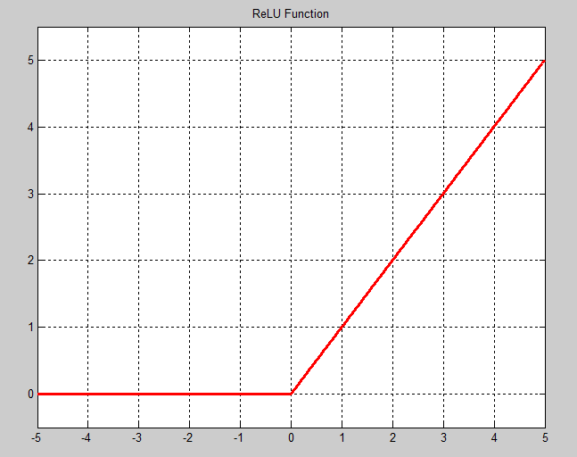
2.2.1 ReLU / Rectified-Linear and Leaky-ReLU
类型: ReLU
例子:
layer {
  name: "relu1"
  type: "ReLU"
  bottom: "conv1"
  top: "conv1"
}
可选参数:
- negative_slope [default 0]: 指定输入值小于零时的输出。
ReLU是目前使用做多的激励函数,主要因为其收敛更快,并且能保持同样效果。标准的ReLU函数为max(x, 0),而一般为当x > 0时输出x,但x <= 0时输出negative_slope。RELU层支持in-place计算,这意味着bottom的输出和输入相同以避免内存的消耗。
2.2.2 Sigmoid
类型:Sigmoid
例子:
layer {
name: "encode1neuron"
bottom: "encode1"
top: "encode1neuron"
type: "Sigmoid"
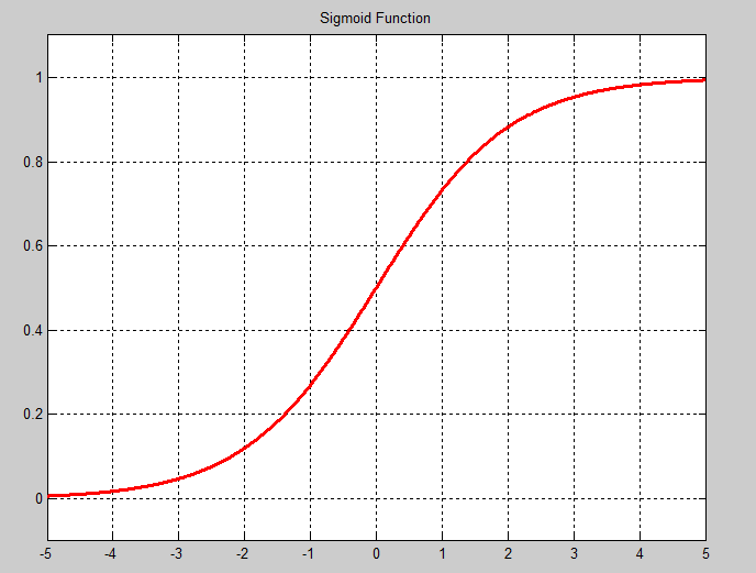
}Sigmoid层通过 sigmoid(x) 计算每一个输入x的输出,函数如下图。
2.2.3 TanH / Hyperbolic Tangent
类型: TanH
例子:
layer {
name: "layer"
bottom: "in"
top: "out"
type: "TanH"
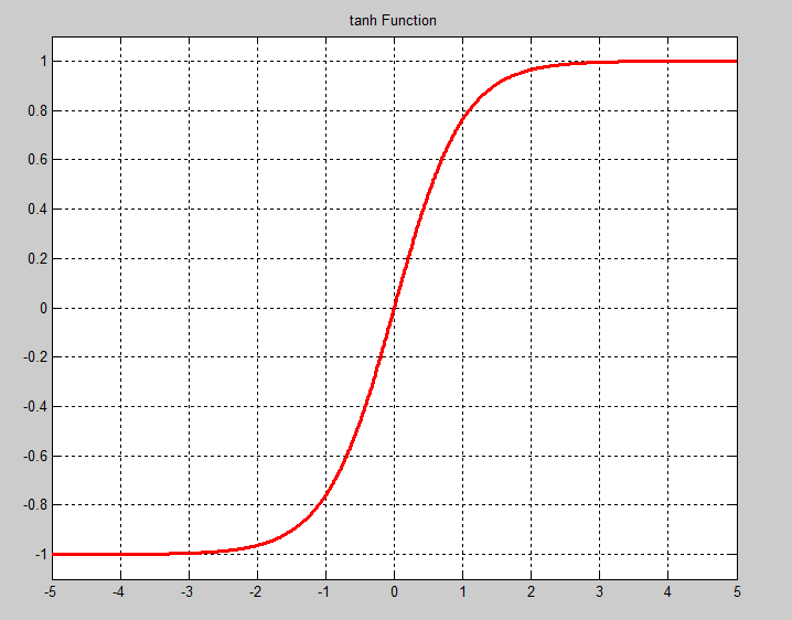
}TanH层通过 tanh(x) 计算每一个输入x的输出,函数如下图。请注意sigmoid函数和TanH函数在纵轴上的区别。sigmoid函数将实数映射到(0,1)。TanH将实数映射到(-1,1)。
2.2.4 Absolute Value
类型: AbsVal
例子:
layer {
  name: "layer"
  bottom: "in"
  top: "out"
  type: "AbsVal"
}
ABSVAL层通过 abs(x) 计算每一个输入x的输出。
2.2.5 Power
类型: Power
例子:
layer {
  name: "layer"
  bottom: "in"
  top: "out"
  type: "Power"
  power_param {
    power: 1
    scale: 1
    shift: 0
  }
}
可选参数:
power [default 1]
scale [default 1]
shift [default 0]
POWER层通过 (shift + scale * x) ^ power计算每一个输入x的输出。
2.2.6 BNLL
类型: BNLL
例子:
layer {
  name: "layer"
  bottom: "in"
  top: "out"
  type: BNLL
}
BNLL (binomial normal log likelihood) 层通过 log(1 + exp(x)) 计算每一个输入x的输出。
2.3. 视觉层(vision_layers)
2.3.1 卷积层(Convolution)
类型:Convolution
例子:
layers {
    name: "conv1"
    type: CONVOLUTION
    bottom: "data"
    top: "conv1"
    blobs_lr: 1               # learning rate multiplier for the filters
    blobs_lr: 2               # learning rate multiplier for the biases
    weight_decay: 1           # weight decay multiplier for the filters
    weight_decay: 0           # weight decay multiplier for the biases
    convolution_param {
        num_output: 96        # learn 96 filters
        kernel_size: 11       # each filter is 11x11
        stride: 4             # step 4 pixels between each filter application
        weight_filler {
            type: "gaussian"  # initialize the filters from a Gaussian
            std: 0.01         # distribution with stdev 0.01 (default mean: 0) }
            bias_filler {
                type: "constant" # initialize the biases to zero (0)
                value: 0
            }
        }
    }
}blobs_lr: 学习率调整的参数,在上面的例子中设置权重学习率和运行中求解器给出的学习率一样,同时是偏置学习率为权重的两倍。
weight_decay:
卷积层的重要参数
必须参数:
num_output (c_o):过滤器的个数
kernel_size (or kernel_h and kernel_w):过滤器的大小(也就是所谓“核”的大小)。
建议参数:
- weight_filler [default type: ‘constant’ value: 0]:参数的初始化方法
可选参数:
bias_filler:偏置的初始化方法
bias_term [default true]:指定是否是否开启偏置项
pad (or pad_h and pad_w) [default 0]:指定在输入的每一边加上多少个像素
stride (or stride_h and stride_w) [default 1]:指定过滤器的步长
group (g) [default 1]: 如果g>1,那么将每个滤波器都限定只与某个输入的子集有关联。换句话说,将输入分为g组,同时将输出也分为g组。那么第i组输出只与第i组输入有关。
通过卷积后的大小变化:
输入:
- n×ci×hi×wi
输出:
- n×co×ho×wo
其中: ho=(hi+2×padh−kernelh)/strideh+1 。 wo 通过同样的方法计算。
2.3.2 池化层(Pooling)
类型:Pooling
例子:
layers {
    name: "pool1"
    type: POOLING
    bottom: "conv1"
    top: "pool1"
    pooling_param {
        pool: MAX
        kernel_size: 3 # pool over a 3x3 region
        stride: 2 # step two pixels (in the bottom blob) between pooling regions
    }
}
卷积层的重要参数
必需参数:
- kernel_size (or kernel_h and kernel_w):过滤器的大小
可选参数:
pool [default MAX]:pooling的方法,目前有MAX, AVE, 和STOCHASTIC三种方法
pad (or pad_h and pad_w) [default 0]:指定在输入的每一遍加上多少个像素
stride (or stride_h and stride_w) [default 1]:指定过滤器的步长
通过池化后的大小变化:
输入:
- n×ci×hi×wi
输出:
- n×co×ho×wo
其中: ho=(hi+2×padh−kernelh)/strideh+1 。 wo 通过同样的方法计算。
2.3.3 Local Response Normalization (LRN)
类型:LRN
可选参数:
local_size [default 5]:对于cross channel LRN为需要求和的邻近channel的数量;对于within channel LRN为需要求和的空间区域的边长;
alpha [default 1]:scaling参数;
beta [default 5]:指数;
norm_region [default ACROSS_CHANNELS]: 选择LRN实现的方法:1. ACROSS_CHANNELS ;2. WITHIN_CHANNEL
LRN(Local Response Normalization)是对一个局部的输入区域进行的归一化。有两种不同的形式:1. ACCROSS_CHANNEL;2. WITHIN_CHANNEL。其实很好从字面上进行理解。第一种方法综合了不同的channel,而在一个channel里面只取1*1(所以size是 localsize×1×1 )。而在第二种方法中,不在channel方向上扩展,只在单一channel上进行空间扩展(所以size是 1×localsize×localsize )。
计算公式:对每一个输入除以 (1+(α/n)⋅∑ix2i)β
在这里,参数 α 是scaling参数,参数 β 是指数。而参数 n 对应local region的大小。
2.4. 损失层(Loss Layers)
深度学习是通过最小化输出和目标的Loss来驱动学习。
2.4.1 Softmax
类型: SoftmaxWithLoss
关于Softmax的内容,可以参考我之前的博客:【机器学习】Softmax Regression简介。Softmax Loss层应用于多标签分类。对于输入,计算了multinomial logistic loss。在概念上近似等于一个Softmax层加上一个multinomial logistic loss层。但在梯度的计算上更加稳定。
2.4.2 Sum-of-Squares / Euclidean
类型: EuclideanLoss
Euclidean loss层计算了两个输入差的平方和:
2.4.3 Hinge / Margin
类型: HingeLoss
例子:
L1 Normlayers {
    name: "loss"
    type: HINGE_LOSS
    bottom: "pred"
    bottom: "label"
}
L2 Normlayers {
    name: "loss"
    type: HINGE_LOSS
    bottom: "pred"
    bottom: "label"
    top: "loss"
    hinge_loss_param {
        norm: L2
    }
}
可选参数:
- norm [default L1]: 选择L1或者L2范数
输入:
- n×c×h×w Predictions
- n×1×1×1 Labels
输出
- 1×1×1×1 Computed Loss
2.4.4 Sigmoid Cross-Entropy
类型:SigmoidCrossEntropyLoss
2.4.5 Infogain
类型:InfoGainLoss
2.4.6 Accuracy and Top-k
类型:Accuracy
用来计算输出和目标的正确率,事实上这不是一个loss,而且没有backward这一步。
2.5. 一般层(Common Layers)
2.5.1 全连接层 Inner Product
类型:InnerProduct
例子:
layer {
  name: "fc8"
  type: "InnerProduct"
  # learning rate and decay multipliers for the weights
  param { lr_mult: 1 decay_mult: 1 }
  # learning rate and decay multipliers for the biases
  param { lr_mult: 2 decay_mult: 0 }
  inner_product_param {
    num_output: 1000
    weight_filler {
      type: "gaussian"
      std: 0.01
    }
    bias_filler {
      type: "constant"
      value: 0
    }
  }
  bottom: "fc7"
  top: "fc8"
}
必要参数:
- num_output (c_o):过滤器的个数
可选参数:
weight_filler [default type: ‘constant’ value: 0]:参数的初始化方法
bias_filler:偏置的初始化方法
bias_term [default true]:指定是否是否开启偏置项
通过全连接层后的大小变化:
输入:
n×ci×hi×wi
输出:
n×co×1×1
2.5.2 Splitting
类型:Split
Splitting层可以把一个输入blob分离成多个输出blobs。这个用在当需要把一个blob输入到多个输出层的时候。
2.5.3 Flattening
类型:Flatten
Flatten层是把一个输入的大小为n * c * h * w变成一个简单的向量,其大小为 n * (c*h*w) * 1 * 1。
2.5.4 Reshape
类型:Reshape
例子:
  layer {
    name: "reshape"
    type: "Reshape"
    bottom: "input"
    top: "output"
    reshape_param {
      shape {
        dim: 0  # copy the dimension from below
        dim: 2
        dim: 3
        dim: -1 # infer it from the other dimensions
      }
    }
  }
输入:单独的一个blob,可以是任意维;
输出:同样的blob,但是它的维度已经被我们人为地改变,维度的数据由reshap_param定义。
可选参数:
- shape
Reshape层被用于改变输入的维度,而不改变输入的具体数据。就像Flatten层一样。只是维度被改变而已,这个过程不涉及数据的拷贝。
输出的维度由ReshapeParam proto控制。可以直接使用数字进行指定。设定输入的某一维到输出blob中去。此外,还有两个数字值得说一下:
0 直接从底层复制。例如,如果是底层是一个2在它的第一维,那么顶层在它的第一维也有一个2。
-1 从其他的数据里面推测这一维应该是多少。
2.5.5 Concatenation
类型:Concat
例子:
layer {
  name: "concat"
  bottom: "in1"
  bottom: "in2"
  top: "out"
  type: "Concat"
  concat_param {
    axis: 1
  }
}
可选参数:
- axis [default 1]:0代表链接num,1代表链接channels
通过全连接层后的大小变化:
输入:从1到K的每一个blob的大小: ni×ci×h×w
输出:
如果axis = 0: (n1+n2+...+nK)×c1×h×w ,需要保证所有输入的 ci 相同。
如果axis = 1: n1×(c1+c2+...+cK)×h×w ,需要保证所有输入的n_i 相同。
通过Concatenation层,可以把多个的blobs链接成一个blob。
2.5.6 Slicing
类型:Slice
例子:
layer {
  name: "slicer_label"
  type: "Slice"
  bottom: "label"
  ## Example of label with a shape N x 3 x 1 x 1
  top: "label1"
  top: "label2"
  top: "label3"
  slice_param {
    axis: 1
    slice_point: 1
    slice_point: 2
  }
}
Slice层可以将输入层变成多个输出层。这些输出层沿一个给定的维度存在。axis指定了目标的轴,slice_point则指定了选择维度的序号。
2.5.7 Elementwise Operations
类型:Eltwise
2.5.8 Argmax
类型:ArgMax
2.5.9 Softmax
类型:Softmax
2.5.10 Mean-Variance Normalization
类型:MVN
3. 后语
结合官方文档,再加画图和看代码,终于对整个layer层有了个基本认识:data负责输入,vision负责卷积相关的计算,neuron和common负责中间部分的数据计算,而loss是最后一部分,负责计算反向传播的误差。具体的实现都在src/caffe/layers里面,慢慢再研究研究。
在这些抽象的基类头文件里,看起来挺累,好在各种搜索,也能学到一些技巧,如,巧用宏定义来简写C,C++代码,使用模板方法,将有大量重复接口和参数的类抽象为一个宏定义,达到简化代码的目的。
4. 参考资料
[1] caffe官方网站
[2] caffe:layer catalogue
[3] MatConvnet Tutorial
[4] MatConvnet Manual
[5] Deep Learning Tutorial
2015/1/4 于 浙大


 1958
1958

 被折叠的 条评论
为什么被折叠?
被折叠的 条评论
为什么被折叠?
 到【灌水乐园】发言


