图像gray（flat） patch 的SNR计算，噪声水平估计

原创已于 2022-08-05 17:12:11 修改

· 1.6k 阅读

7 ·

版权

文章标签：

#python #计算机视觉 #opencv

于 2022-07-08 09:35:45 首次发布

图像处理算法专栏收录该内容

94 篇文章

订阅专栏

实验一一张图像不同亮度区域的噪声水平

在很多论文中假设图像 0 均值高斯噪声，同一张图像无论亮度，每个像素的噪声水平都是一样的，然而实际不是这样，所以后面才有高斯-泊松噪声模型。下面这个小实验来验证一下。

噪声类型有很多，常见的有高斯噪声和 shot(符合泊松分布，又称泊松噪声)

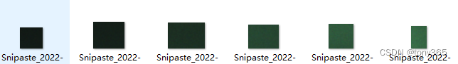
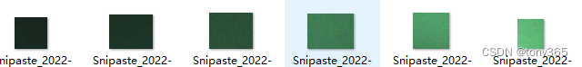
这里截取 raw图 24色卡的 patch20,patch21,patch22中的灰块，不同亮度的色块噪声强度应该时不一样，看下实验结果是否如此。
patch22
patch21
patch20
然后计算每个灰块的 rgb分布，计算均值，方差以及 snr

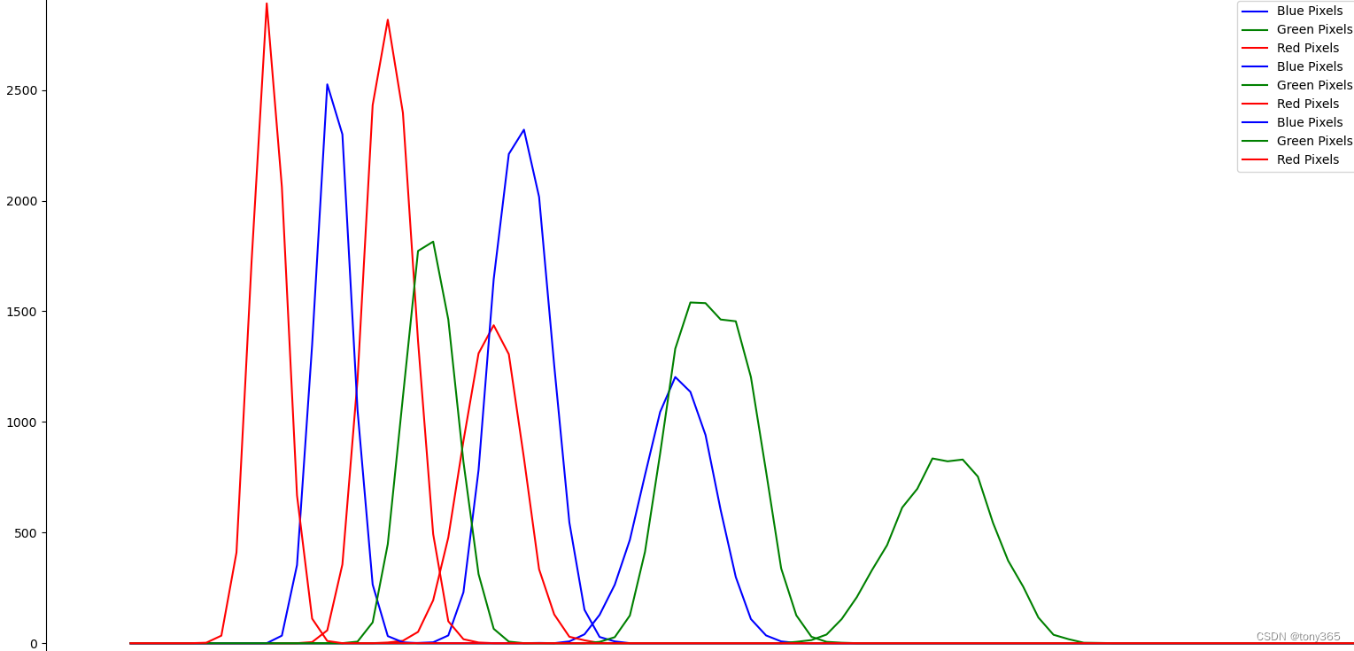
三个patch 各自 rgb的 hist如下
三个patch各自的rgb分布
计算结果如下：
请添加图片描述
截图中sigma是标准差，图片中标注错了。

从数据看，可以说明什么呢，噪声看起来类似高斯噪声，但是不同亮度的patch 噪声水平是不同的，说明噪声不是独立与图像的。而是随着亮度增加噪声方差（水平）也跟着增加，另外hist可以看出高斯分布并不标准，这应该都是泊松噪声的影响。

下面是计算的code

import cv2
import numpy as np
from matplotlib import pyplot as plt

def cal_gray_snr(mu, sigma):
    return 10 * np.log10((mu**2) / (sigma**2))

# 上面的计算snr的方法有误，下面的
# https://www.cnblogs.com/qrlozte/p/5340216.html
def cal_gray_snr2(im):
    im = im.astype(np.float64)
    im = im / 255

    a = np.sum(im*im, axis=(0, 1))
    m = np.mean(im, axis=(0, 1)).reshape([1,1,3])

    b = np.sum((im-m)**2, axis=(0, 1))

    return 10*np.log10(a / b)

def cal_gray_psnr2(im):
    n = im.shape[0] * im.shape[1]
    im = im.astype(np.float64)
    im = im / 255

    m = np.mean(im, axis=(0, 1)).reshape([1,1,3])

    b = np.sum((im-m)**2, axis=(0, 1))

    return 10*np.log10(n / b)

if __name__ == "__main__":

    file = r'D:\dataset\dang_yingxiangzhiliangceshi\snr\2patch2.png'
    image = cv2.imread(file)
    file = r'D:\dataset\dang_yingxiangzhiliangceshi\snr\2patch3.png'
    image2 = cv2.imread(file)
    file = r'D:\dataset\dang_yingxiangzhiliangceshi\snr\2patch4.png'
    image3 = cv2.imread(file)


    mu = np.mean(image, axis=(0,1))
    sigma = np.std(image, axis=(0,1))
    mu2 = np.mean(image2, axis=(0,1))
    sigma2 = np.std(image2, axis=(0,1))
    mu3 = np.mean(image3, axis=(0,1))
    sigma3 = np.std(image3, axis=(0,1))

    t = cal_gray_snr(mu, sigma)
    t2 = cal_gray_snr(mu2, sigma2)
    t3 = cal_gray_snr(mu3, sigma3)
    print(mu, sigma, t, t.mean())
    print(mu2, sigma2, t2, t2.mean())
    print(mu3, sigma3, t3, t3.mean())
    snr = cal_gray_snr2(image)
    snr2 = cal_gray_snr2(image2)
    snr3 = cal_gray_snr2(image3)
    print('snr :')
    print(snr, snr.mean(), cal_gray_psnr2(image))
    print(snr2, snr2.mean(), cal_gray_psnr2(image2))
    print(snr3, snr3.mean(), cal_gray_psnr2(image3))
    colors = ('blue','green','red')
    label = ("Blue", "Green", "Red")
    for count,color in enumerate(colors):
        histogram = cv2.calcHist([image],[count],None,[256],[0,256])
        plt.plot(histogram,color = color, label=label[count]+str(" Pixels"))
    for count,color in enumerate(colors):
        histogram = cv2.calcHist([image2],[count],None,[256],[0,256])
        plt.plot(histogram,color = color, label=label[count]+str(" Pixels"))
    for count,color in enumerate(colors):
        histogram = cv2.calcHist([image3],[count],None,[256],[0,256])
        plt.plot(histogram,color = color, label=label[count]+str(" Pixels"))

    plt.title("Histogram Showing Number Of Pixels Belonging To Respective Pixel Intensity", color="crimson")
    plt.ylabel("Number Of Pixels", color="crimson")
    plt.xlabel("Pixel Intensity", color="crimson")
    plt.legend(numpoints=1, loc="best")
    plt.show()

实验二多张不同ISO图像的噪声水平

这里进行如下实验，分别设置 iso 的倍数为1，2，3. 得到24色卡的灰块patch, 计算每个灰块的 snr
iso为1倍时的 6个patch
在这里插入图片描述
iso为2倍时的6个patch

在这里插入图片描述
iso为3倍时的6个patch

计算每个patch 每个通道的snr 和 snr.mean()
iso 1
[28.29987974 27.49178948 29.53692843] 28.442865879546407
[28.92858405 29.15168355 30.71157171] 29.59727977170645
[30.08926321 30.48947076 30.09068842] 30.223140797873857
[31.39342856 31.26194743 30.71822399] 31.124533329485928
[28.77417059 27.68122584 28.04556752] 28.16698798410329
[28.90366269 27.63406401 28.59977507] 28.37916725661869
iso 2
[26.93171222 26.52456257 27.76157229] 27.072615696211297
[27.20195513 27.15525802 27.9756152 ] 27.444276114155816
[28.43930221 29.26027784 28.65266255] 28.784080868521915
[29.80552016 30.63488256 28.88727897] 29.775893895820488
[28.77189499 28.39681035 27.72472941] 28.297811582905208
[27.35266233 28.27187127 27.95320909] 27.85924756073598
iso 3
[24.45524367 24.63813555 25.37541484] 24.822931352690574
[25.05417468 26.48662864 25.86998991] 25.803597744865424
[27.66651116 28.5901588 27.46090744] 27.905859134218417
[29.45153691 29.37756144 28.30282574] 29.04397469511198
[25.57301453 25.89656988 25.76413814] 25.74457418333576
[27.08026178 28.2832994 27.63958125] 27.667714142869567

可以得到如下结论（只能说大概如此，以来截取patch 大小位置不一，二来光线不均匀，三来噪声的分布实际情况是比较复杂的。）
1）随着iso增大，信噪比降低
2）同样的iso下不同亮度的色块信噪比时一致的。（亮度大的区域，均值大，方差也大，最后信噪比变化不大）
3）同样的iso下，同一张图像不同亮度的噪声强度时不一样的，亮块noise level比较大（方差比较大），也就是泊松噪声的影响