OBB-最小外接矩形包围框-原理-代码实现

前言

• 定义：OBB是相对于物体方向对齐的包围盒，不再局限于坐标轴对齐，因此包围点云时更加紧密。
• 优点：能够更好地贴合物体形状，减少空白区域。
• 缺点：计算较为复杂，需要计算物体的主方向，进行旋转和缩放变换。

算法原理

实现OBB通常涉及以下步骤：

1. 计算凸包（Convex Hull）
2. 使用主成分分析（Principal Component Analysis，简称PCA）找到最佳的旋转方向
3. 根据这些方向确定包围盒的边界

步骤一：计算凸包

凸包是一组点的最小凸多边形，包含所有点，并且所有点都在多边形的边界上或内部。可以使用scipy库中的ConvexHull函数来计算。

import numpy as np
from scipy.spatial import ConvexHull
# 生成数据
mean = [0, 0]
cov = [[3, 1], [1, 2]]
points = np.random.multivariate_normal(mean, cov, 300)

# 计算凸包
convex_hull = ConvexHull(points)
# 可视化
plt.figure(figsize=(10, 8))
plt.scatter(points[:, 0], points[:, 1], s=10, alpha=0.5, label='Points')

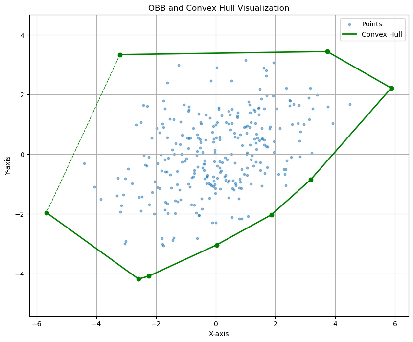
图 展示了图包得到的最外层点及其点之间的连线

步骤二：主成分分析（PCA）

PCA可以帮助我们找到数据的主方向。通过分析凸包顶点的协方差矩阵，我们可以得到主要的方向，这些方向定义了OBB的方向。

from sklearn.decomposition import PCA

pca = PCA(n_components=2)
pca.fit(points[convex_hull.vertices])  # 仅对凸包顶点进行PCA

步骤三：根据PCA方向计算OBB

根据PCA的结果，我们可以确定OBB的方向。然后，我们需要计算在这些方向上点的投影，以此来确定矩形的边界。

# OBB计算函数
def compute_obb(points):
    # 使用PCA找到数据的主成分方向
    pca = PCA(n_components=2)
    pca.fit(points)
    
    # 得到主轴
    eigen_vectors = pca.components_
    eigen_values = pca.explained_variance_
    
    # 将点投影到主轴上
    projected_points = np.dot(points, eigen_vectors.T)
    
    # 计算包围盒的边界
    min_proj = np.min(projected_points, axis=0)
    max_proj = np.max(projected_points, axis=0)
    
    # 通过主轴和包围盒的边界重构OBB顶点
    obb_vertices = np.array([
        [min_proj[0], min_proj[1]],
        [min_proj[0], max_proj[1]],
        [max_proj[0], max_proj[1]],
        [max_proj[0], min_proj[1]]
    ])
    
    # 将OBB顶点从PCA空间转换回原始空间
    obb_vertices = np.dot(obb_vertices, eigen_vectors)
    
    return obb_vertices
obb_vertices = compute_obb(points)

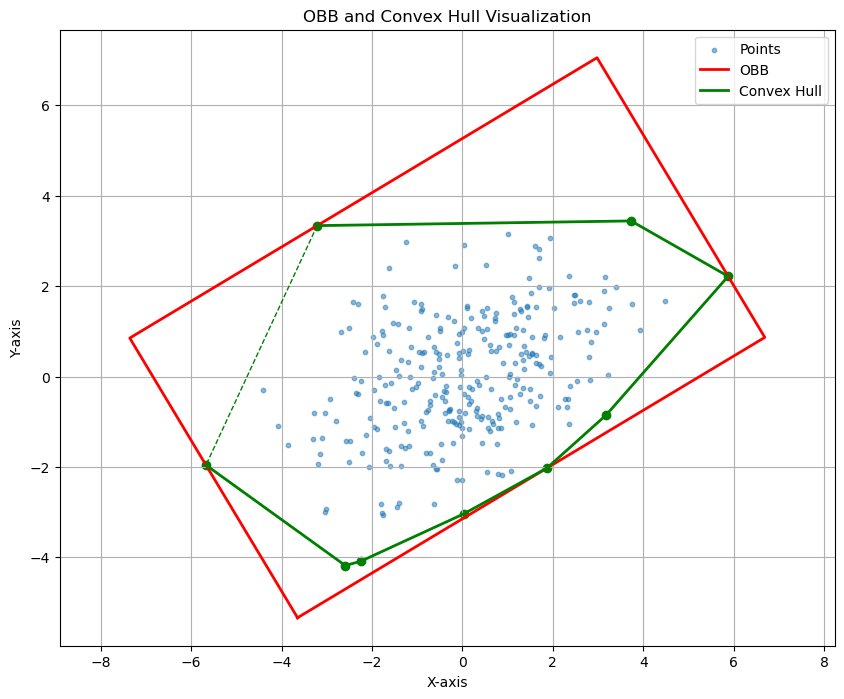
上述代码定义了计算OBB的整个过程，从计算凸包到应用PCA，最后确定边界框的角。每步都是基于数学原理进行建模，确保能找到最合适的包围盒。

完整代码

import numpy as np
import matplotlib.pyplot as plt
from sklearn.decomposition import PCA
from scipy.spatial import ConvexHull

# OBB计算函数
def compute_obb(points):
    # 使用PCA找到数据的主成分方向
    pca = PCA(n_components=2)
    pca.fit(points)
    
    # 得到主轴
    eigen_vectors = pca.components_
    eigen_values = pca.explained_variance_
    
    # 将点投影到主轴上
    projected_points = np.dot(points, eigen_vectors.T)
    
    # 计算包围盒的边界
    min_proj = np.min(projected_points, axis=0)
    max_proj = np.max(projected_points, axis=0)
    
    # 通过主轴和包围盒的边界重构OBB顶点
    obb_vertices = np.array([
        [min_proj[0], min_proj[1]],
        [min_proj[0], max_proj[1]],
        [max_proj[0], max_proj[1]],
        [max_proj[0], min_proj[1]]
    ])
    
    # 将OBB顶点从PCA空间转换回原始空间
    obb_vertices = np.dot(obb_vertices, eigen_vectors)
    
    return obb_vertices

np.random.seed(42)
mean = [0, 0]
cov = [[3, 1], [1, 2]]
points = np.random.multivariate_normal(mean, cov, 300)

# 计算OBB顶点
obb_vertices = compute_obb(points)

# 计算凸包
convex_hull = ConvexHull(points)

# 可视化点云、OBB和凸包
plt.figure(figsize=(10, 8))
plt.scatter(points[:, 0], points[:, 1], s=10, alpha=0.5, label='Points')

# 绘制OBB
obb_polygon = np.vstack([obb_vertices, obb_vertices[0]])  # 闭合OBB多边形
plt.plot(obb_polygon[:, 0], obb_polygon[:, 1], 'r-', linewidth=2, label='OBB')

# 绘制凸包
for simplex in convex_hull.simplices:
    plt.plot(points[simplex, 0], points[simplex, 1], 'g--', linewidth=1)

plt.plot(points[convex_hull.vertices, 0], points[convex_hull.vertices, 1], 'g-', linewidth=2, label='Convex Hull')
plt.scatter(points[convex_hull.vertices, 0], points[convex_hull.vertices, 1], color='green')

plt.title('OBB and Convex Hull Visualization')
plt.xlabel('X-axis')
plt.ylabel('Y-axis')
plt.legend()
plt.axis('equal')
plt.grid(True)
plt.show()

利用Open3D使用OBB算法

import open3d as o3d
import numpy as np

# 读取点云 txt 文件，假设文件名为 'point_cloud.txt'
file_path = './data/5.txt'

# 使用 numpy 读取数据
point_cloud_data = np.loadtxt(file_path)

# 提取点的坐标 (x, y, z) 和颜色 (r, g, b)
points = point_cloud_data[:, :3]
colors = point_cloud_data[:, 3:] / 255.0  # Open3D expects colors in [0, 1] range

# 创建 Open3D 点云对象
pcd = o3d.geometry.PointCloud()
pcd.points = o3d.utility.Vector3dVector(points)
pcd.colors = o3d.utility.Vector3dVector(colors)


# 计算AABB（轴对齐包围盒）
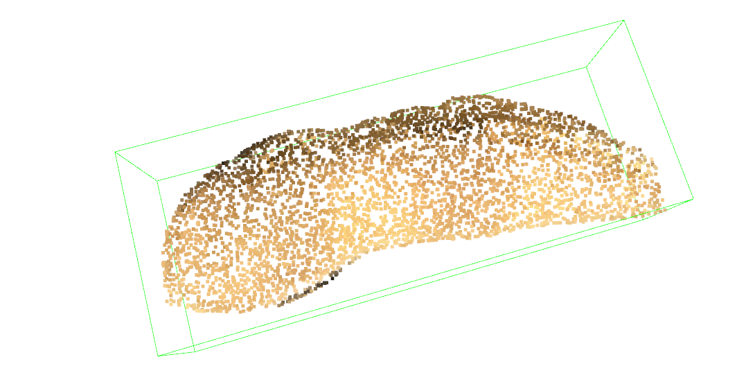
obb = pcd.get_oriented_bounding_box()
axis = o3d.geometry.TriangleMesh.create_coordinate_frame()


# 可视化点云和AABB
obb.color = (0, 1, 0)  
o3d.visualization.draw_geometries([pcd,obb])

可视化结果：