横向扩展 纵向扩展 数据库_通过正则化扩展您的回归库

横向扩展 纵向扩展 数据库

You can also read this article on GitHub. This GitHub repository includes everything you need to run the analyses yourself.

您还可以在GitHub上阅读本文。 该GitHub存储库包含您自己运行分析所需的一切。

介绍 (Introduction)

For many data scientists, the basic workhorse model is multiple linear regression. It serves as the first port of call in many analyses, and as the benchmark for more complicated models. One of its strengths is the easy interpretability of the resulting coefficients, something that especially neural networks struggle with. However, linear regression is not without its challenges. In this article, we focus on one particular challenge: dealing with large sets of features. Specific issues with large datasets are how to select the relevant features for our model, how to combat overfitting and how to deal with correlated features.

对于许多数据科学家而言，基本的工作模型是多元线性回归。 在许多分析中，它充当呼叫的第一站，并作为更复杂模型的基准。 它的优点之一是所得系数的易于解释性，尤其是神经网络难以解决的问题。 但是，线性回归并非没有挑战。 在本文中，我们将重点放在一个特殊的挑战上：处理大量功能。 大型数据集的特定问题是如何为模型选择相关特征，如何应对过度拟合以及如何处理相关特征。

Regularisation is a very potent technique that helps with the above-mentioned issues. Regularisation does this by expanding the normal least squares goal or loss function with a term which limits the size of coefficients. The main goal of this article is to get you familiar with regularisation and the advantages it offers.

正则化是一种非常有效的技术，可以解决上述问题。 正则化通过用限制系数大小的项扩展正常最小二乘法目标或损失函数来实现。 本文的主要目的是使您熟悉正则化及其提供的优点。

In this article you will learn about the following topics:

在本文中，您将学习以下主题：

• What regularisation is in more detail and why it is worthwhile to use
  什么更正则化以及为什么值得使用
• What different types of regularisation there are, and what the terms L1- and L2-norm mean in this context
  有哪些不同类型的正则化，以及在这种情况下术语L1-和L2-norm的含义是什么
• How to practically use regularisation
  如何实际使用正则化
• How to generate features for our regularised regression using tsfresh
  如何使用tsfresh为我们的正则回归生成特征
• How to interpret and visualise the coefficients of the regularised regression
  如何解释和可视化正则回归的系数
• How to optimize the regularisation strength using crossvalidation
  如何使用交叉验证优化正则化强度
• How to visualise the outcomes of the crossvalidation
  如何可视化交叉验证的结果

We will start this article off with a more theoretical introduction to regularisation, and finish up with a practical example.

我们将从更理论上介绍正则化开始本文，并以一个实际示例结束。

为什么要使用正则化，什么是规范？ (Why use regularisation and what are norms?)

The following figure shows a green and a blue function fitted to the red observations (attribution). Both functions perfectly fit the red observations, and we really have no good way of choosing either of the functions using a loss function.

下图显示了适合于红色观测值的绿色和蓝色功能( 归因 )。 这两个函数都非常适合红色观测值，并且我们真的没有使用损失函数选择任何一个函数的好方法。

Not being able to choose either of these functions means that our problem is underdetermined. In regression, two factors increase the degree of underdetermination: multicollinearity (correlated features) and the number of features. In a situation with a small amount of handcrafted features this can often be controlled for manually. However, in more data driven approaches we often work with a lot of (correlated) features of which we do not a priori know which ones will work well. To combat undetermination we need to add information to our problem. The mathematical term for adding information to our problem is regularisation.

无法选择这些功能中的任何一个都意味着我们的问题尚未得到确定 。 在回归中， 两个因素增加了不确定性的程度 ：多重共线性(相关特征)和特征数量。 在手工功能较少的情况下，通常可以手动控制。 但是，在更多的数据驱动方法中，我们经常使用许多(相关的)功能，而我们事先都不知道哪个功能会很好。 为了消除不确定性，我们需要向我们的问题中添加信息。 为我们的问题添加信息的数学术语是正则化 。

A very common way in regression to perform regularisation is by expanding the loss function with additional terms. Tibshirani (1997) proposed to add the total size of the coefficients to the loss function in a method called Lasso. A mathematical way to express the total size of the coefficients is using a so called *norm*:

回归执行正则化的一种非常常见的方法是通过使用其他项扩展损失函数。 Tibshirani(1997)提出了用拉索方法将系数的总大小添加到损失函数中。 一种表达系数总大小的数学方法是使用所谓的* norm *：

where the p value determines what kind of norm we use. A p value of 1 is called an L1 norm, a value of 2 a L2 norm, etcetera. Now that we have a mathetical epxression for the norm, we can expand the least squares loss function we normally use in regression:

p值决定我们使用哪种范数。 p值1称为L1范数，值2称为L2范数，等等。 现在我们有了数学上的范数，我们可以扩展我们通常在回归中使用的最小二乘损失函数：

note that we use an L2 norm here, and that we also expressed the squared difference part of the loss function using a L2 norm. In addition, lambda is the regularisation strength. The regularisation strength determines how strongly the focus will be on limiting coefficient size versus the squared difference part of the loss function. Note that the norm term introduces a bias into the regression, with the major upside of reducing the variance in the model.

请注意，我们在这里使用L2范数，并且我们也使用L2范数表示损失函数的平方差部分。 另外，lambda是正则化强度。 正则强度确定焦点将集中在限制系数大小相对于损失函数平方差的大小上。 注意，范数项在回归中引入了偏差，主要的好处是减少模型中的方差。

Regression including a L2 norm is called Ridge regression (sklearn). Ridge regression reduces the variance in the prediction, making it more stable and less prone to overfitting. In addition, the reduction in variance also combats the variance introduced by multicollinearity.

包含L2范数的回归称为里奇回归 ( sklearn )。 岭回归减少了预测中的方差，使其更稳定并且不太容易拟合。 此外，方差的减少还可以抵抗由多重共线性引入的方差 。

When we add an L1 norm in the loss function, this is called Lasso (sklearn). Lasso goes a step further than Ridge regression in reducing the coefficient size, all the way down to zero. This effectively means that the variable drops out of the model, and thus lasso performs feature selection. This has a large effect when dealing with highly correlated features (multicollinearity). Lasso tends to pick one of the correlated variables, while Ridge regression balances all features. The feature selection property of Lasso is particularly useful when you have a lot of input features of which you do not know in advance which ones will prove beneficial to the model.

当我们在损失函数中添加L1范数时，这称为Lasso( sklearn )。 在减小系数大小(一直到零)方面，Lasso比Ridge回归更进一步。 这实际上意味着变量退出模型，因此套索执行特征选择。 当处理高度相关的特征(多重共线性)时，这会产生很大的影响。 套索倾向于选择相关变量之一，而岭回归则平衡所有特征。 当您有很多输入特征而您事先不知道哪些对模型有利时，Lasso的特征选择属性特别有用。

If you want to blend Lasso and Ridge regression, you can add both an L1 and L2 norm to the loss function. This is called Elastic Net regularisation. With the theoretical part out of the way, let us get into the practical application of regularisation.

如果要混合使用Lasso和Ridge回归，可以将L1和L2范数都添加到损失函数中。 这称为Elastic Net正则化 。 除去理论部分，让我们进入正则化的实际应用。

使用正则化的示例 (Example use of regularisation)

用例 (The use case)

Humans are quite good recognizing sounds. Based on audio alone we are able to distinguish between things like cars, voices, and guns. If someone is particularly experienced they may even be able to tell you what kind of car the sound belongs to. In this example case we will build a regularised logistic regression model to recognize drum sounds.

人类在识别声音方面非常出色。 仅基于音频，我们就能够区分汽车，声音和枪支。 如果某人特别有经验，他们甚至可以告诉您声音属于哪种汽车。 在此示例中，我们将建立一个规则化的逻辑回归模型来识别鼓声。

数据集 (The dataset)

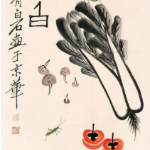
The basis for our model is a set of 75 drum samples, 25 of each type of drum: kick drum, snare drum and tom. Each drum sample is stored in a wav file, for example:

我们模型的基础是一组75个鼓样本，每种鼓中有25个： 踢鼓 ， 军鼓和鼓 。 每个鼓样本都存储在一个wav文件中，例如：

high res version 高分辨率版本

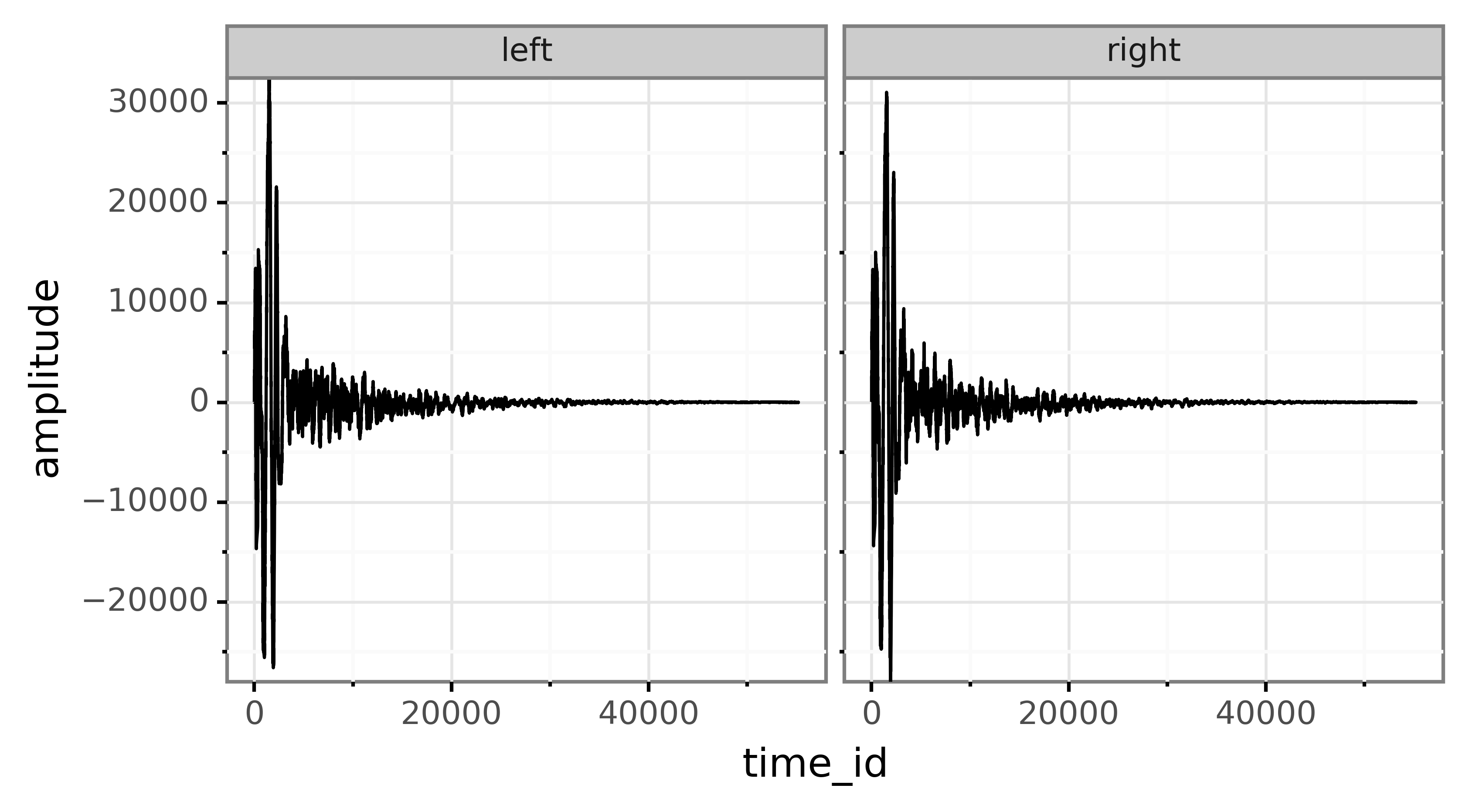
The wav file is stereo and contains two channels: left and right. The file contains a waveform over time with time on the x-axis and amplitude on the y-axis. The amplitude essentially lists how the conus of the loudspeaker should vibrate in order to replicate the sound that is stored in the file.

wav文件是立体声文件，包含两个通道：左和右。 该文件包含随时间变化的波形，x轴为时间，y轴为振幅。 振幅实质上列出了扬声器的圆锥体应如何振动以复制存储在文件中的声音。

The following code constructs a DataFrame with all 75 drum samples:

以下代码使用所有75个鼓样本构造一个DataFrame ：

The extra function audio_to_dataframe can be found in the helper_functions.py file in the github repo of the article.

额外的函数audio_to_dataframe可以在本文的github存储库的helper_functions.py文件中找到。

使用tsfresh生成功能 (Generating features using tsfresh)

To fit a supervised model, sklearn needs two datasets: a samples x features matrix (or DataFrame) with our features and a samples vector with the labels. As we already have the labels (all_labels), we focus our efforts on the feature matrix. As we want our model to make a prediction for each sound file, each row in the feature matrix should contain all features for one sound file. The next challenge then is to come up with the features we want to use. For example, the bass drum probably has more bass frequencies in its sounds. We could therefore run an FFT over all samples and isolate the bass frequency into a feature.

为了适应监督模型，sklearn需要两个数据集：具有我们特征的samples x features矩阵(或DataFrame)和具有标签的samples向量。 由于我们已经有了标签( all_labels )，因此我们将精力集中在特征矩阵上。 因为我们希望模型为每个声音文件做出预测，所以特征矩阵中的每一行都应包含一个声音文件的所有特征。 然后，下一个挑战是提出我们要使用的功能。 例如，大鼓的声音中可能有更多的低音频率。 因此，我们可以对所有样本运行FFT，并将低音频率隔离为一个特征。

Taking this manual feature engineering approach can be very labour intensive, and has a strong risk of excluding important features. tsfresh (docs) is a Python package which greatly speeds this process up. The package generates hundreds of potential features based on timeseries data, and also includes a means to preselect relevant features. Having hundreds of features stresses the importance of using some kind of regularisation in this case.

采用这种手动特征工程方法可能会非常费力，并且有排除重要特征的巨大风险。 tsfresh ( docs )是一个Python软件包，可大大加快此过程。 该程序包根据时间序列数据生成数百个潜在特征，并且还包括一种预选相关特征的方法。 在这种情况下，具有数百个功能强调了使用某种正则化的重要性。

To get familiair with tsfresh we first generate a small number of features by using the MinimalFCParameters setting:

为了使用tsfresh获得功能，我们首先使用MinimalFCParameters设置生成少量功能：

which leaves us with 11 features. We use the extract_relevant_features function to allow tsfresh to preselect features that make sense given the labels and potential features generated. In this minimal case, tsfresh looks at each of the sound files as identified by the file_id column and generates features such as the standard deviation of the amplitude, the mean amplitude and more.

剩下11个功能。 我们使用extract_relevant_features函数允许tsfresh预先选择在给定标签和可能生成的特征的情况下有意义的特征。 在这种最小的情况下，tsfresh会查看file_id列标识的每个声音文件，并生成诸如幅度的标准偏差，平均幅度等等的特征。

But the strength of tsfresh comes when we generate a lot more features. Here we use the efficient settings to save some time in contrast to the complete setting. Note I read the result from a saved pickled DataFrame which has been generated using the generate_drum_model.py script available in the github repo. I did this to save time as it takes around 10 minutes on my 12 thread machine to calculate the efficient features.

但是，当我们生成更多功能时，tsfresh的优势就会显现。 与完整的设置相比，这里我们使用有效的设置来节省一些时间。 注意我从保存的腌制DataFrame中读取了结果，该数据是使用github存储库中的generate_drum_model.py脚本generate_drum_model.py 。 我这样做是为了节省时间，因为在我的12线程计算机上大约需要10分钟才能计算出有效的功能。

This greatly expands the number of features from 11 to 327. Now the features include autocorrelation across several possible lags, FFT components and linear and non-linear trends, etcetera, etcetera. These features provide a very expansive learning space for our regularised regression model to work with.

这将特征的数量从11个大大扩展到327个。现在，这些特征包括跨多个可能滞后的自相关，FFT分量以及线性和非线性趋势等。 这些功能为我们的正则回归模型提供了非常广阔的学习空间。

拟合正则回归模型 (Fitting the regularised regression model)

Now that we have a set of input features and the required labels, we can go ahead and fit our regularised regression model. We use the logistic regression model from sklearn:

现在，我们有了一组输入功能和所需的标签，我们可以继续进行拟合并拟合我们的正则回归模型。 我们使用sklearn的逻辑回归模型：

and use the following settings:

并使用以下设置：

• we set the penalty to l1, i.e. we use regularisation with an L1 norm.

  我们将惩罚设置为l1 ，即我们使用具有L1范数的正则化。

• we set multi_class equal to one-versus-rest (ovr). This means that our model consists of three sub-models in our case, one for each of the possible types of drums. When predicting with the overall model, we simply choose the model which performs best.

  我们设置multi_class等于one-versus-rest ( ovr )。 这意味着我们的模型由三个子模型组成，每种子鼓都有一个子模型。 在使用整体模型进行预测时，我们只需选择效果最佳的模型即可。

• we use the saga solver to fit our loss function. There are many more available, but saga has a complete set of features.

  我们使用saga求解器来拟合我们的损失函数。 还有更多可用的功能，但saga具有完整的功能集。

• C is set to 1 for now, where C equals 1/regularisation strength. Note that the sklearn Lasso implementation uses 𝛼, which equals 1/2C. Because I find 𝛼 a more intuitive measure, we will use that throughout the remainder of the article.

  现在将C设置为1，其中C等于1/regularisation strength 。 注意，sklearn Lasso实现使用uses，它等于1/2C 。 因为我发现𝛼更直观的度量，所以我们将在本文的其余部分中使用它。

• tol and max_iter are set to acceptable defaults.

  tol和max_iter设置为可接受的默认值。

Based on these settings we perform a number of experiments. First we will compare the performance of a models based on both the small and larger amount of tsfresh features. After that we will focus on fitting the regularisation strength using crossvalidation, and wrap up with a more general discussion of the performance of the fitted model.

基于这些设置，我们执行了许多实验。 首先，我们将比较基于少量和大量tsfresh功能的模型的性能。 之后，我们将集中于使用交叉验证拟合正则化强度，并以更一般性的讨论来讨论拟合模型的性能。

最小的tsfresh vs高效 (Minimal tsfresh vs efficient)

Our first analysis tests the hypothesis that using more generated tsfresh features leads to a better model. To test this, we fit a model using both the minimal and efficient tsfresh features. We judge model performance via the accuracy the model has on a test set. We repeat this 20 times to get a sense for the variance in the accuracy due to the randomness in choosing training and test set:

我们的第一个分析检验了以下假设：使用更多生成的tsfresh功能可以得到更好的模型。 为了对此进行测试，我们使用最小和有效的tsfresh功能对模型进行拟合。 我们通过模型在测试集上的准确性来判断模型的性能。 由于选择训练和测试集的随机性，我们重复了20次以了解准确性的差异：

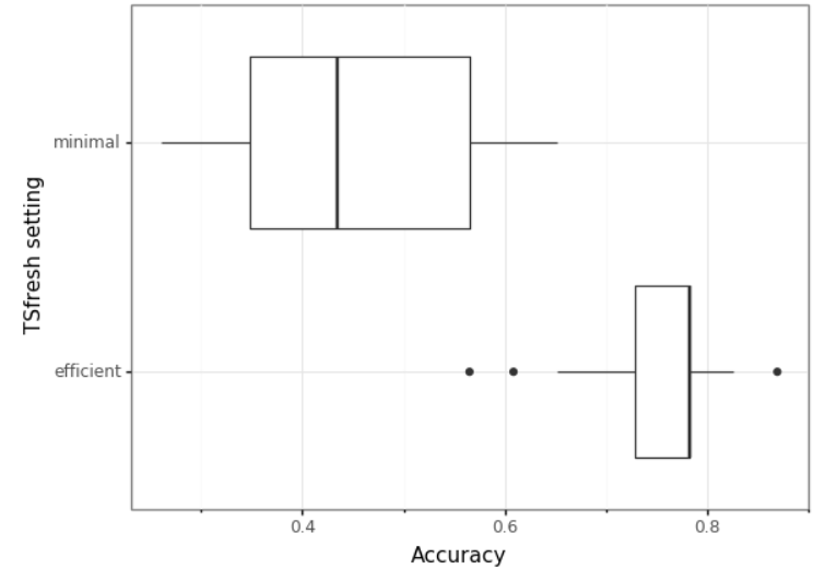
The resulting boxplot clearly shows that the efficient tsfresh variables show a much higher mean accuracy of 0.75 versus the 0.4 of the minimal features based model. This confirms our hypothesis, and we will use the efficient features in the rest of this article.

所得的箱线图清楚地表明，有效的tsfresh变量显示出0.75的平均准确度，而基于最小特征的模型的平均准确度则为0.4。 这证实了我们的假设，并且我们将在本文的其余部分中使用有效的功能。

通过交叉验证选择正则化强度 (Selecting regularisation strength through crossvalidation)

One of the major choices we have to make when using regularisation is the regularisation strength. Here we use crossvalidation to test the accuracy of a range of potential values of C. Conviniently, sklearn includes a function which performs this analysis for logistic regression: LogisticRegressionCV. It essentially has the same interface as LogisticRegression, but you can pass along a list of potential C values to test. For details regarding the code I refer to the generate_drum_model.py script on github, and we load the results here from disk to save time:

使用正则化时，我们必须做出的主要选择之一是正则化强度。 在这里，我们使用交叉验证来测试C的潜在值范围的准确性。方便地，sklearn包括一个执行此逻辑回归分析的函数： LogisticRegressionCV 。 它本质上具有与LogisticRegression相同的接口，但是您可以传递潜在的C值列表进行测试。 有关代码的详细信息，请参阅github上的generate_drum_model.py脚本，我们在这里从磁盘加载结果以节省时间：

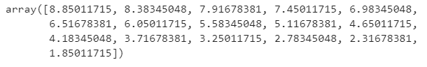
Note we use l1_min_c to get the minimum C value for which the model will still contains non-zero coefficients. Then we add a log scale between 0 and 7 on top of that to end up with 16 potential C values. I do not have a good reason for these numbers, I simply reused them from the tutorial in the l1_min_c link. Transformed to 𝛼α regularisation strength and taking the log10 value (for readability) we end up with:

请注意，我们使用l1_min_c来获取模型仍将包含非零系数的最小C值。 然后，我们在其上添加一个介于0到7之间的对数刻度，以得到16个潜在的C值。 对于这些数字，我没有充分的理由，我只是在l1_min_c链接的教程中重复使用了它们。 转换为𝛼α正则化强度并采用log10值(出于可读性)，我们最终得到：

This spans a nice range of regularisation strength as we will see in the interpretation of the results.

正如我们在结果解释中所看到的，这涵盖了很好的正则化强度范围。

The crossvalidation selected the following 𝛼 values:

交叉验证选择了以下𝛼个值：

Note we have three values, one for each submodel (kick-model, tom-model, snare-model). Here we see that a regularisation strength of around 6 is judged to be optimal (C = 4.5e-07).

注意，我们有三个值，每个子模型一个值(踢模型，tom模型，小军鼓模型)。 在这里，我们看到正则化强度被认为是最佳的(C = 4.5e-07 )。

基于简历结果的模型进一步解释 (Further interpretation of the model based on CV results)

The cv_result object contains a lot more data regarding the crossvalidation then the fitted regularisation strength. Here we first look at the coefficients in the crossvalidated models, and what path they followed under changing regularisation strength. Note we use the plot_coef_paths function from the helper_functions.py file on github:

cv_result对象包含更多的关于交叉验证的数据，而不是拟合的正则化强度。 在这里，我们首先查看交叉验证模型中的系数，以及它们在变化的正则化强度下所遵循的路径。 请注意，我们使用github上helper_functions.py文件中的plot_coef_paths函数：

high res version 高分辨率版本

Note we see 5 lines in the plot as by default we perform 5-fold crossvalidation. In addition, we focus on the kick sub-model. The following observations are interesting in this figure:

请注意，我们在图中看到5条线，因为默认情况下我们执行5倍交叉验证。 另外，我们关注kick子模型。 以下观察在这个图中很有趣：

• Increasing the regularisation strength decreases the size of the coefficients. This is exactly what regularisation is supposed do to, but it is nice that the results support this.
  增加正则强度会减小系数的大小。 这正是正则化应该执行的操作，但是结果很好地支持了这一点。
• Increasing the regularisation strength reduces the variation between the fitted coefficients for the folds (lines are closer together). The is in line with the goal of regularisation: reducing variance in the model and fight underdetermination. However, the variation between folds can still be quite dramatic.
  增加正则强度会减小折线的拟合系数之间的差异(线条靠得更近)。 这符合正则化的目标：减少模型中的方差并消除不确定性。 但是，折痕之间的差异仍然很大。
• The overall coefficient size drops for the later coefficients. So, earlier coefficients are most important in the model.
  对于随后的系数，总系数大小下降。 因此，较早的系数在模型中最重要。
• For the crossvalidated regularisation strength (6) quite a number of coefficients drop out of the model. Of the 327 potential features generated by tsfresh, only around 10 are selected for the final model.
  对于交叉验证的正则化强度(6)，很多系数会从模型中剔除。 tsfresh生成的327个潜在特征中，最终模型仅选择了大约10个。
• Many of the influential variables are fft components. This makes sense intuitively as the difference between the drum samples is centered around certain frequencies (bass drum -> low freq, snare -> high freq).
  许多有影响力的变量都是fft的组成部分。 由于鼓采样之间的差异集中在某些频率上(低音鼓->低频率，军鼓->高频率)，这在直观上是有意义的。

These observations paint the picture that the regularised regression works as intended, but there is certainly room for improvement. In this case I suspect that having 25 samples of each type of drum is the main limiting factor.

这些观察结果描绘了正则回归按预期工作的情况，但是肯定还有改进的空间。 在这种情况下，我怀疑每种类型的鼓具有25个样本是主要的限制因素。

Apart from looking at the coefficients and how they change, we can also look at the overal accuracy of the sub-models versus the regularisation strength. Note that we use the plot_reg_strength_vs_score plot from helper_functions.py which you can find on github.

除了查看系数及其变化方式之外，我们还可以查看子模型的总体准确性与正则化强度之间的关系。 请注意，我们使用来自helper_functions.py的plot_reg_strength_vs_score图，您可以在github上找到它。

high res version 高分辨率版本

Note that the accuracy covers not a line but an area because we have an accuracy score for each fold in the crossvalidation. Observations in this figure:

请注意，准确性不覆盖直线，而是覆盖区域，因为我们对交叉验证中的每一折都有准确性得分。 该图的观察结果：

• The kick model performs best overall with a very low minimum accuracy at the fitted regularisation strength (6 -> 0.95).
  踢腿模型在拟合的正则强度(6-> 0.95)下，以极低的最低精度表现出最佳的整体效果。
• The tom model performs worst with a substantially lower minimum and maximum accuracy.
  汤姆模型以最差的最小和最大准确度表现最差。
• Performance peaks between a regularisation strength of 5–6, which is in line with the selected values. With a smaller strength, I suspect too much noise from the superfluous variables left in the model, after that the regularisation takes out too much relevant information.
  性能在5–6的正则化强度之间达到峰值，这与所选值一致。 在强度较小的情况下，我怀疑模型中剩余的多余变量会产生过多的噪声，此后正则化会去除过多的相关信息。

结论：我们的正则回归模型的性能 (Conclusion: performance of our regularised regression model)

Based on the accuracy scores from the cross-validation I conclude that we are quite successful at generating a drum sound recognition model. Especially the kick drum is easy to distinguish from the other two drum types. Regularised regression also adds a lot of value to the model, and reduces the overall variance of the model. Finally, tsfresh shows a lot of potential in generating features from these kinds of time series based datasets.

根据交叉验证的准确性得分，我得出结论，我们在生成鼓声识别模型方面非常成功。 尤其是脚鼓易于与其他两种鼓类型区分开。 正则回归还为模型增加了很多价值，并减少了模型的总体差异。 最后，tsfresh显示了从这些基于时间序列的数据集中生成特征的巨大潜力。

Potential avenues to improve the model are:

改进模型的潜在途径是：

• Generate more potential input features using tsfresh. For this analysis, I used the efficient settings, but more elaborate settings are possible.
  使用tsfresh生成更多潜在的输入要素。 在此分析中，我使用了有效的设置，但可以进行更精细的设置。
• Use more drum samples as input to the model.
  使用更多的鼓样本作为模型的输入。

翻译自: https://towardsdatascience.com/expanding-your-regression-repertoire-with-regularisation-903d2c9f7b28

横向扩展 纵向扩展 数据库