三人决斗_使用深度q决斗学习为厄运建立进攻性AI代理

三人决斗

介绍 (Introduction)

Over the last few articles, we’ve discussed and implemented Deep Q-learning (DQN)and Double Deep Q Learning (DDQN) in the VizDoom game environment and evaluated their performance. Deep Q-learning is a highly flexible and responsive online learning approach that utilizes rapid intra-episodic updates to it’s estimations of state-action (Q) values in an environment in order to maximize reward. Double Deep Q-Learning builds upon this by decoupling the networks responsible for action selection and TD-target calculation in order to minimize Q-value overestimation, a problem particularly evident when earlier on in the training process, when the agent has yet to fully explore the majority of possible states.

在过去的几篇文章中,我们已经在VizDoom游戏环境中 讨论实现了 深度Q学习 (DQN)和双深度Q学习 (DDQN),并评估了它们的性能。 深度Q学习是一种高度灵活且响应Swift的在线学习方法,它利用快速的内部事件更新对其在环境中的状态作用(Q)值的估计,以最大化回报。 Double Deep Q-Learning以此为基础,通过将负责动作选择和TD目标计算的网络解耦,以最大程度地降低Q值高估,这一问题在训练过程的较早阶段,即代理商尚未完全探索时尤其明显。大多数可能的状态。

Inherently, using a single state-action value in judging a situation demands exploring and learning the effects of an action for every single state, resulting in an inherent hindrance to the model’s generalization capabilities. Moreover, not all states are equally relevant within the context of the environment.

本质上,使用单个状态-动作值来判断情况需要探索和学习每个单个状态的动作效果,从而对模型的泛化能力产生了固有的阻碍。 而且,并非所有状态在环境中都具有同等的相关性。

Image for post
Preprocessed Frame from our previous agent trained in Pong.
来自我们 先前在Pong培训的 代理商的预处理框架。

Recall our Pong environment from our earlier implementations. Immediately after our agent hits the ball, the value of moving left or right is negligible, as the ball must first travel to the opponent and be returned towards the player. Calculating state-action values at this point to use for training may disrupt the convergence of our agent as a result. Ideally, we would like to be able to identify the value of each action without learning its effects specific to each state, in order to encourage our agent to focus on selecting actions relevant to the environment.

回忆一下我们以前的实现中的 Pong环境。 在我们的探员击球后,向左或向右移动的值立即可以忽略不计,因为球必须首先行进对手并返回球员。 计算此时用于训练的状态行动值可能会破坏我们代理的收敛性。 理想情况下,我们希望能够在不了解每个行为特定于每个状态的影响的情况下,识别每个行为的价值,以鼓励我们的代理商专注于选择与环境相关的行为。

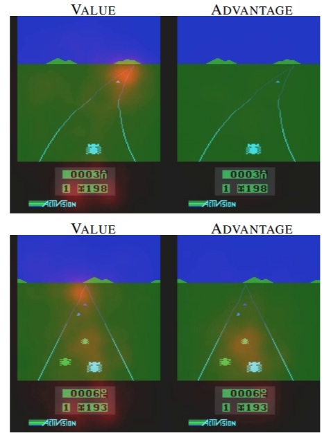
Dueling Deep Q-Learning (henceforth DuelDQN) addresses these shortcomings by splitting the DQN network output into two streams: a value stream and an advantage (or action) stream. In doing so, we partially decouple the overall state-action evaluation process. In their seminal paper, Van Hasselt et. al presented a visualization of how DuelDQN affected agent performance in the Atari game Enduro, demonstrating how the agent could learn to focus on separate objectives. Notice how the value stream has learned to focus on the direction of the road, while the advantage stream has learned to focus on the immediate obstacles in front of the agent. In essence, we have gained a level of short-term and medium-term foresight through this approach.

决斗深度Q学习(以下简称DuelDQN)通过将DQN网络输出分为两个流来解决这些缺点:价值流和优势(或行动)流。 在此过程中,我们将整个状态动作评估过程部分地分离了。 Van Hasselt等人在其开创性论文中。 他等人展示了Atel游戏Enduro中DuelDQN如何影响特工性能的可视化,演示了特工如何学会专注于单独的目标。 请注意,价值流如何学会专注于道路的方向,而优势流如何学会专注于代理商前方的直接障碍。 从本质上讲,我们通过这种方法获得了短期和中期的预测。

Image for post

To calculate the Q-value of a state-action, we then utilize the advantage function is to tell us the relative importance of an action. The subtraction of the average advantage, calculated across all possible actions in a state, is used to find the relative advantage of our interested action.

为了计算状态动作的Q值,我们利用优势函数来告诉我们动作的相对重要性。 对状态中所有可能的动作计算得出的平均优势的减法用于查找我们感兴趣的动作的相对优势。

Image for post
The Q-value of a state-action according to the DuelDQN architecture.
根据DuelDQN体系结构的状态动作的Q值。

Intuitively, we have partially decoupled the action and state-value estimation processes in order to gain a more reliable appraisal of the environment.

直观上,我们已将操作和状态值估计过程部分分离,以便获得对环境的更可靠评估。

实作 (Implementation)

We’ll be implementing our approach in the same VizDoomgym scenario as in our last article, Defend The Line, with the same multi-objective conditions. Some characteristics of the environment include:

我们将在与上一篇文章Defend The Line相同的VizDoomgym场景中使用相同的多目标条件来实现我们的方法。 环境的一些特征包括:

  • An action space of 3: fire, turn left, and turn right. Strafing is not allowed.

    3个动作空间,开火,向左转,再向右转。 不允许散装。
  • Brown monsters that shoot fireballs at the player with a 100% hit rate.

    以100%的命中率向玩家射击火球的棕色怪物。
  • Pink monsters that attempt to move close in a zig-zagged pattern to bite the player.

    试图以锯齿状移动的方式咬住玩家的粉红色怪物。
  • Respawned monsters can endure more damage.

    重生的怪物可以承受更多的伤害。
  • +1 point for killing a monster.

    杀死怪物+1点。
  • - 1 point for dying.

    -1点死亡。
Image for post
Initial state of the “Defend The Line Scenario”
“捍卫线路情景”的初始状态

Our Google Colaboratory implementation is written in Python utilizing Pytorch, and can be found on the GradientCrescent Github. Our approach is based on the approach detailed in Tabor’s excellent Reinforcement Learning course. As our DuelDQN implementation is similar to our previous vanilla DQN implementation, the overall high-level workflow is shared, and won’t be repeated here.

我们的Google合作实验室实现是使用Pytorch用Python编写的,可以在GradientCrescent Github上找到 我们的方法基于Tabor出色的强化学习课程中详述的方法。 由于我们的DuelDQN实现类似于我们以前的原始DQN实现,因此共享了整个高级工作流程, 在此不再赘述

Let’s start by importing all of the necessary packages, including the OpenAI and Vizdoomgym environments. We’ll also install the AV package necessary for Torchvision, which we’ll use for visualization. Note that the runtime must be restarted after installation is complete before the rest of the notebook can be executed.

首先,导入所有必需的软件包,包括OpenAI和Vizdoomgym环境。 我们还将安装Torchvision所需的AV软件包,并将其用于可视化。 请注意,安装完成后必须重新启动运行系统,然后才能执行笔记本的其余部分。

#Visualization cobe for running within Colab
!sudo apt-get update
!sudo apt-get install build-essential zlib1g-dev libsdl2-dev libjpeg-dev nasm tar libbz2-dev libgtk2.0-dev cmake git libfluidsynth-dev libgme-dev libopenal-dev timidity libwildmidi-dev unzip# Boost libraries
!sudo apt-get install libboost-all-dev# Lua binding dependencies
!apt-get install liblua5.1-dev
!sudo apt-get install cmake libboost-all-dev libgtk2.0-dev libsdl2-dev python-numpy git
!git clone https://github.com/shakenes/vizdoomgym.git
!python3 -m pip install -e vizdoomgym/!pip install av

Next, we initialize our environment scenario, inspect the observation space and action space, and visualize our environment.

接下来,我们初始化环境方案,检查观察空间和动作空间,并可视化我们的环境。

import gym
import vizdoomgymenv = gym.make('VizdoomDefendLine-v0')
n_outputs = env.action_space.n
print(n_outputs)observation = env.reset()import matplotlib.pyplot as pltfor i in range(22):
if i > 20:
print(observation.shape)
plt.imshow(observation)
plt.show()observation, _, _, _ = env.step(1)

Next, we’ll define our preprocessing wrappers. These are classes that inherit from the OpenAI gym base class, overriding their methods and variables in order to implicitly provide all of our necessary preprocessing. We’ll start defining a wrapper to repeat every action for a number of frames, and perform an element-wise maxima in order to increase the intensity of any actions. You’ll notice a few tertiary arguments such as fire_first and no_ops — these are environment-specific, and of no consequence to us in Vizdoomgym.

接下来,我们将定义预处理包装器。 这些类继承自OpenAI Gym基础类,并覆盖其方法和变量,以隐式提供我们所有必要的预处理。 我们将开始定义一个包装器,以便在多个帧中重复每个动作,并执行逐个元素的最大值,以增加任何动作的强度。 您会注意到一些三级参数,例如fire_firstno_ops ,它们是特定于环境的,在Vizdoomgym中对我们没有影响。

class RepeatActionAndMaxFrame(gym.Wrapper):
#input: environment, repeat
#init frame buffer as an array of zeros in shape 2 x the obs space
def __init__(self, env=None, repeat=4, clip_reward=False, no_ops=0,
fire_first=False):
super(RepeatActionAndMaxFrame, self).__init__(env)
self.repeat = repeat
self.shape = env.observation_space.low.shape
self.frame_buffer = np.zeros_like((2, self.shape))
self.clip_reward = clip_reward
self.no_ops = no_ops
self.fire_first = fire_first
def step(self, action):
t_reward = 0.0
done = False
for i in range(self.repeat):
obs, reward, done, info = self.env.step(action)
if self.clip_reward:
reward = np.clip(np.array([reward]), -1, 1)[0]
t_reward += reward
idx = i % 2
self.frame_buffer[idx] = obs
if done:
break
max_frame = np.maximum(self.frame_buffer[0], self.frame_buffer[1])
return max_frame, t_reward, done, info
def reset(self):
obs = self.env.reset()
no_ops = np.random.randint(self.no_ops)+1 if self.no_ops > 0 else 0
for _ in range(no_ops):
_, _, done, _ = self.env.step(0)
if done:
self.env.reset()
if self.fire_first:
assert self.env.unwrapped.get_action_meanings()[1] == 'FIRE'
obs, _, _, _ = self.env.step(1)
self.frame_buffer = np.zeros_like((2,self.shape))
self.frame_buffer[0] = obs
return obs

Next, we define the preprocessing function for our observations. We’ll make our environment symmetrical by converting it into the standardized Box space, swapping the channel integer to the front of our tensor, and resizing it to an area of (84,84) from its original (320,480) resolution. We’ll also greyscale our environment, and normalize the entire image by dividing by a constant.

接下来,我们为观察定义预处理功能。 通过将其转换为标准化的Box空间,将通道整数交换到张量的前端,并将其大小调整为原始分辨率(320,480)到(84,84),可以使环境对称。 我们还将对环境进行灰度处理,并通过除以一个常数来标准化整个图像。

class PreprocessFrame(gym.ObservationWrapper):
#set shape by swapping channels axis
#set observation space to new shape using gym.spaces.Box (0 to 1.0)
def __init__(self, shape, env=None):
super(PreprocessFrame, self).__init__(env)
self.shape = (shape[2], shape[0], shape[1])
self.observation_space = gym.spaces.Box(low=0.0, high=1.0,
shape=self.shape, dtype=np.float32)
def observation(self, obs):
new_frame = cv2.cvtColor(obs, cv2.COLOR_RGB2GRAY)
resized_screen = cv2.resize(new_frame, self.shape[1:],
interpolation=cv2.INTER_AREA)
new_obs = np.array(resized_screen, dtype=np.uint8).reshape(self.shape)
new_obs = new_obs / 255.0
return new_obs

Next, we create a wrapper to handle frame-stacking. The objective here is to help capture motion and direction from stacking frames, by stacking several frames together as a single batch. In this way, we can capture position, translation, velocity, and acceleration of the elements in the environment. With stacking, our input adopts a shape of (4,84,84,1).

接下来,我们创建一个包装器来处理框架堆叠。 此处的目的是通过将几个帧作为一个批处理一起堆叠来帮助捕获堆叠帧的运动和方向。 通过这种方式,我们可以捕获环境中元素的位置,平移,速度和加速度。 通过堆叠,我们的输入采用(4,84,84,1)的形状。

class StackFrames(gym.ObservationWrapper):
#init the new obs space (gym.spaces.Box) low & high bounds as repeat of n_steps. These should have been defined for vizdooom
#Create a return a stack of observations
def __init__(self, env, repeat):
super(StackFrames, self).__init__(env)
self.observation_space = gym.spaces.Box( env.observation_space.low.repeat(repeat, axis=0),
env.observation_space.high.repeat(repeat, axis=0),
dtype=np.float32)
self.stack = collections.deque(maxlen=repeat)
def reset(self):
self.stack.clear()
observation = self.env.reset()
for _ in range(self.stack.maxlen):
self.stack.append(observation)
return np.array(self.stack).reshape(self.observation_space.low.shape)
def observation(self, observation):
self.stack.append(observation)
return np.array(self.stack).reshape(self.observation_space.low.shape)

Finally, we tie all of our wrappers together into a single make_env() method, before returning the final environment for use.

最后,在返回最终使用环境之前,我们将所有包装器绑定到单个make_env()方法中。

def make_env(env_name, shape=(84,84,1), repeat=4, clip_rewards=False,
no_ops=0, fire_first=False):
env = gym.make(env_name)
env = PreprocessFrame(shape, env)
env = RepeatActionAndMaxFrame(env, repeat, clip_rewards, no_ops, fire_first)
env = StackFrames(env, repeat)
return env

Next, let’s define our model, a deep Q-network featuring two outputs for the dueling architecture. This is essentially a three layer convolutional network that takes preprocessed input observations, with the generated flattened output fed to a fully-connected layer, after which the output is then split into the value stream (with a single node output), and the advantage stream (with a node output corresponding to the number of actions in the environment).

接下来,让我们定义我们的模型,即一个深度Q网络,该网络具有两个用于决斗架构的输出。 这本质上是一个三层卷积网络,接受预处理的输入观测值,并将生成的展平输出馈送到全连接层,然后将输出分成值流(具有单节点输出)和优势流(节点输出对应于环境中的动作数)。

Note there are no activation layers here, as the presence of one would result in a binary output distribution. Our loss is the squared difference of our estimated Q-value of our current state-action and our predicted state-action value. We then attach the RMSProp optimizer to minimize our loss during training.

注意这里没有激活层,因为一个激活层会导致二进制输出分布。 我们的损失是我们当前状态行为的估计Q值和预测状态行为值的平方差。 然后,我们附加RMSProp优化器,以最大程度地减少训练过程中的损失。

import os
import torch as T
import torch.nn as nn
import torch.nn.functional as F
import torch.optim as optim
import numpy as npclass DeepQNetwork(nn.Module):
def __init__(self, lr, n_actions, name, input_dims, chkpt_dir):
super(DeepQNetwork, self).__init__()
self.checkpoint_dir = chkpt_dir
self.checkpoint_file = os.path.join(self.checkpoint_dir, name) self.conv1 = nn.Conv2d(input_dims[0], 32, 8, stride=4)
self.conv2 = nn.Conv2d(32, 64, 4, stride=2)
self.conv3 = nn.Conv2d(64, 64, 3, stride=1) fc_input_dims = self.calculate_conv_output_dims(input_dims) self.fc1 = nn.Linear(fc_input_dims,1024)
self.fc2 = nn.Linear(1024, 512)
#Here we split the linear layer into the State and Advantage streams
self.V = nn.Linear(512, 1)
self.A = nn.Linear(512, n_actions) self.optimizer = optim.RMSprop(self.parameters(), lr=lr) self.loss = nn.MSELoss()
self.device = T.device('cuda:0' if T.cuda.is_available() else 'cpu')
self.to(self.device) def calculate_conv_output_dims(self, input_dims):
state = T.zeros(1, *input_dims)
dims = self.conv1(state)
dims = self.conv2(dims)
dims = self.conv3(dims)
return int(np.prod(dims.size())) def forward(self, state):
conv1 = F.relu(self.conv1(state))
conv2 = F.relu(self.conv2(conv1))
conv3 = F.relu(self.conv3(conv2))
# conv3 shape is BS x n_filters x H x W
conv_state = conv3.view(conv3.size()[0], -1)
# conv_state shape is BS x (n_filters * H * W)
flat1 = F.relu(self.fc1(conv_state))
flat2 = F.relu(self.fc2(flat1)) V = self.V(flat2)
A = self.A(flat2) return V, A def save_checkpoint(self):
print('... saving checkpoint ...')
T.save(self.state_dict(), self.checkpoint_file) def load_checkpoint(self):
print('... loading checkpoint ...')
self.load_state_dict(T.load(self.checkpoint_file))

Recall that the update function for dueling deep Q-learning requires the following:

回想一下,进行深度Q学习的更新功能需要以下条件:

  • The current state s

    目前的状态s

  • The current action a

    目前的行动

  • The reward following the current action r

    按照目前的行动R上的奖励

  • The next state s’

    下一状态S'

  • The next action a’

    接下来的行动”

To supply these parameters in meaningful quantities, we need to evaluate our current policy following a set of parameters and store all of the variables in a buffer, from which we’ll draw data in minibatches during training. Hence, we need a replay memory buffer from which to store and draw observations from.

为了以有意义的数量提供这些参数,我们需要根据一组参数评估当前策略,并将所有变量存储在缓冲区中,在训练过程中,我们将从这些缓冲区中提取数据。 因此,我们需要一个重播内存缓冲区,从中可以存储和提取观察结果。

import numpy as np
class ReplayBuffer(object):
def __init__(self, max_size, input_shape, n_actions):
self.mem_size = max_size
self.mem_cntr = 0
self.state_memory = np.zeros((self.mem_size, *input_shape),
dtype=np.float32)
self.new_state_memory = np.zeros((self.mem_size, *input_shape),
dtype=np.float32)
self.action_memory = np.zeros(self.mem_size, dtype=np.int64)
self.reward_memory = np.zeros(self.mem_size, dtype=np.float32)
self.terminal_memory = np.zeros(self.mem_size, dtype=np.bool)
#Identify index and store the the current SARSA into batch memory def store_transition(self, state, action, reward, state_, done):
index = self.mem_cntr % self.mem_size
self.state_memory[index] = state
self.new_state_memory[index] = state_
self.action_memory[index] = action
self.reward_memory[index] = reward
self.terminal_memory[index] = done
self.mem_cntr += 1 def sample_buffer(self, batch_size):
max_mem = min(self.mem_cntr, self.mem_size)
batch = np.random.choice(max_mem, batch_size, replace=False)
states = self.state_memory[batch]
actions = self.action_memory[batch]
rewards = self.reward_memory[batch]
states_ = self.new_state_memory[batch]
terminal = self.terminal_memory[batch]
return states, actions, rewards, states_, terminal

Next, we’ll define our agent, which differs form our vanilla DQN implementation. Our agent be using an epsilon greedy policy with a decaying exploration rate, in order to maximize exploitation over time. To learn to predict state and advantages values that maximize our cumulative reward, our agent will be using the discounted future rewards obtained by sampling the stored memory.

接下来,我们将定义代理,这与我们的原始DQN实现不同。 我们的代理商正在使用具有逐渐降低的勘探速度的epsilon贪婪策略,以期随着时间的推移最大化开发利用。 为了学习预测最大化我们的累积奖励的状态和优势值,我们的代理商将使用通过对存储的内存进行采样获得的折现的未来奖励。

You’’ll notice that we initialize two copies of our DQN as part of our agent, with methods to copy weight parameters of our original network into a target network. While our vanilla approach utilized this setup to generate stationary TD-targets, the presence of dual streams in our DuelDQN approach adds a layer of complexity to the process:

您会注意到,作为代理的一部分,我们初始化了DQN的两个副本,其中包含将原始网络的权重参数复制到目标网络的方法。 尽管我们的原始方法利用此设置来生成固定的TD目标,但DuelDQN方法中双流的存在为该过程增加了一层复杂性:

  • States, Actions, Rewards, and Next States (SARS) are retrieved from the Replay Memory.

    从重播内存中检索状态,操作,奖励和下一个状态(SARS)。
  • The evaluation network is used to generate the advantage (A_s) and state (V_s) values of the current state .

    评估网络用于生成当前状态的优势( A_s )和状态( V_s )值。

  • The target network is also used to create the advantage (A_s_) and state (V_s_) values of the next state.

    目标网络还用于创建下一个状态的优势( A_s_ )和状态( V_s_ )值。

  • The predicted Q-values are generated by summing the advantage and state values of the current state, and subtracting the mean of the current state advantage value for normalization.

    预测Q值是通过将当前状态的优势和状态值相加,然后减去当前状态优势值的平均值进行归一化而生成的。
  • The target Q-values current state is calculated by summing the advantage and state values of the next state, and subtracting the mean of the next state advantage value for normalization.

    目标Q值当前状态是通过将下一个状态的优势和状态值相加,然后减去下一个状态优势值的平均值进行归一化计算得出的。
  • The TD target is then built by combining the discounted target Q-values with the current state reward.

    然后,通过将折后的目标Q值与当前状态奖励相结合来构建TD目标。
  • A loss function is calculated by comparing the TD-target with the predicted Q-values, which is then used to train the network.

    通过将TD目标与预测的Q值进行比较来计算损失函数,然后将其用于训练网络。
import numpy as np
import torch as T
#from deep_q_network import DeepQNetwork
#from replay_memory import ReplayBufferclass DuelDQNAgent(object):
def __init__(self, gamma, epsilon, lr, n_actions, input_dims,
mem_size, batch_size, eps_min=0.01, eps_dec=5e-7,
replace=1000, algo=None, env_name=None, chkpt_dir='tmp/dqn'):
self.gamma = gamma
self.epsilon = epsilon
self.lr = lr
self.n_actions = n_actions
self.input_dims = input_dims
self.batch_size = batch_size
self.eps_min = eps_min
self.eps_dec = eps_dec
self.replace_target_cnt = replace
self.algo = algo
self.env_name = env_name
self.chkpt_dir = chkpt_dir
self.action_space = [i for i in range(n_actions)]
self.learn_step_counter = 0 self.memory = ReplayBuffer(mem_size, input_dims, n_actions) self.q_eval = DeepQNetwork(self.lr, self.n_actions,
input_dims=self.input_dims,
name=self.env_name+'_'+self.algo+'_q_eval',
chkpt_dir=self.chkpt_dir) self.q_next = DeepQNetwork(self.lr, self.n_actions,
input_dims=self.input_dims,
name=self.env_name+'_'+self.algo+'_q_next',
chkpt_dir=self.chkpt_dir)#Epsilon greedy action selection
def choose_action(self, observation):
if np.random.random() > self.epsilon:
# Add dimension to observation to match input_dims x batch_size by placing in list, then converting to tensor
state = T.tensor([observation],dtype=T.float).to(self.q_eval.device)
#As our forward function now has both state and advantage, fetch latter for actio selection
_, advantage = self.q_eval.forward(state)
action = T.argmax(advantage).item()
else:
action = np.random.choice(self.action_space) return action def store_transition(self, state, action, reward, state_, done):
self.memory.store_transition(state, action, reward, state_, done) def sample_memory(self):
state, action, reward, new_state, done = \
self.memory.sample_buffer(self.batch_size) states = T.tensor(state).to(self.q_eval.device)
rewards = T.tensor(reward).to(self.q_eval.device)
dones = T.tensor(done).to(self.q_eval.device)
actions = T.tensor(action).to(self.q_eval.device)
states_ = T.tensor(new_state).to(self.q_eval.device) return states, actions, rewards, states_, dones def replace_target_network(self):
if self.learn_step_counter % self.replace_target_cnt == 0:
self.q_next.load_state_dict(self.q_eval.state_dict()) def decrement_epsilon(self):
self.epsilon = self.epsilon - self.eps_dec \
if self.epsilon > self.eps_min else self.eps_min def save_models(self):
self.q_eval.save_checkpoint()
self.q_next.save_checkpoint() def load_models(self):
self.q_eval.load_checkpoint()
self.q_next.load_checkpoint()
def learn(self):
if self.memory.mem_cntr < self.batch_size:
return self.q_eval.optimizer.zero_grad() #Replace target network if appropriate
self.replace_target_network() states, actions, rewards, states_, dones = self.sample_memory()
#Fetch states and advantage actions for current state using eval network
#Also fetch the same for next state using target network
V_s, A_s = self.q_eval.forward(states)
V_s_, A_s_ = self.q_next.forward(states_) #Indices for matrix multiplication
indices = np.arange(self.batch_size) #Calculate current state Q-values and next state max Q-value by aggregation, subtracting constant advantage mean
q_pred = T.add(V_s,
(A_s - A_s.mean(dim=1, keepdim=True)))[indices, actions]
q_next = T.add(V_s_,
(A_s_ - A_s_.mean(dim=1, keepdim=True))).max(dim=1)[0] q_next[dones] = 0.0
#Build your target using the current state reward and q_next
q_target = rewards + self.gamma*q_next loss = self.q_eval.loss(q_target, q_pred).to(self.q_eval.device)
loss.backward()
self.q_eval.optimizer.step()
self.learn_step_counter += 1 self.decrement_epsilon()

With all of supporting code defined, let’s run our main training loop. We’ve defined most of this in the initial summary, but let’s recall for posterity.

定义了所有支持代码后,让我们运行主训练循环。 我们已经在初始摘要中定义了大部分内容,但让我们回顾一下后代。

  • For every step of a training episode, we feed an input image stack into our network to generate a probability distribution of the available actions, before using an epsilon-greedy policy to select the next action

    对于训练情节的每个步骤,在使用epsilon-greedy策略选择下一个动作之前,我们将输入图像堆栈输入到网络中以生成可用动作的概率分布。
  • We then input this into the network, and obtain information on the next state and accompanying rewards, and store this into our buffer. We update our stack and repeat this process over a number of pre-defined steps.

    然后,我们将其输入到网络中,并获取有关下一个状态和伴随的奖励的信息,并将其存储到我们的缓冲区中。 我们更新堆栈,并通过许多预定义的步骤重复此过程。
  • At the end of an episode, we feed the next states into our network in order to obtain the next action. We also calculate the next reward by discounting the current one.

    在剧集结束时,我们将下一个状态馈入网络中以获得下一个动作。 我们还通过折现当前奖励来计算下一个奖励。
  • We generate our target y-values through the Q-learning update function mentioned above, and train our network.

    我们通过上述Q学习更新功能生成目标y值,并训练我们的网络。
  • By minimizing the training loss, we update the network weight parameters to output improved state-action values for the next policy.

    通过最大程度地减少训练损失,我们更新了网络权重参数,以便为下一个策略输出改进的状态操作值。
  • We evaluate models by tracking their average score (measured over 100 training steps).

    我们通过跟踪模型的平均得分(超过100个训练步骤来评估)来评估模型。
env = make_env('VizdoomDefendLine-v0')
best_score = -np.inf
load_checkpoint = False
n_games = 2000
agent = DuelDQNAgent(gamma=0.99, epsilon=1.0, lr=0.0001,input_dims=(env.observation_space.shape),n_actions=env.action_space.n, mem_size=5000, eps_min=0.1,batch_size=32, replace=1000, eps_dec=1e-5,chkpt_dir='/content/', algo='DuelDQNAgent',env_name='vizdoogym')if load_checkpoint:
agent.load_models()fname = agent.algo + '_' + agent.env_name + '_lr' + str(agent.lr) +'_'+ str(n_games) + 'games'
figure_file = 'plots/' + fname + '.png'n_steps = 0
scores, eps_history, steps_array = [], [], []for i in range(n_games):
done = False
observation = env.reset() score = 0
while not done:
action = agent.choose_action(observation)
observation_, reward, done, info = env.step(action)
score += reward if not load_checkpoint:
agent.store_transition(observation, action,reward, observation_, int(done))
agent.learn()
observation = observation_
n_steps += 1scores.append(score)
steps_array.append(n_steps)avg_score = np.mean(scores[-100:])if avg_score > best_score:
best_score = avg_score
print('Checkpoint saved at episode ', i)
agent.save_models()print('Episode: ', i,'Score: ', score,' Average score: %.2f' % avg_score, 'Best average: %.2f' % best_score,'Epsilon: %.2f' % agent.epsilon, 'Steps:', n_steps)eps_history.append(agent.epsilon)
if load_checkpoint and n_steps >= 18000:
break

We’ve graphed the average score of our agents together with our episodic epsilon value, across 500, 1000, and 2000 episodes below.

在下面的500、1000和2000集中,我们绘制了代理商的平均得分以及情节ε值。

Image for post
Reward distribution of our agent after 500 episodes.
500集后奖励我们的特工的奖励分配。
Image for post
Reward distribution of our agent after 1000 episodes.
1000集后奖励我们的特工的奖励分配。
Image for post
Reward distribution of our agent after 200 episodes.
200集后奖励我们的经纪人。

Looking at the results and comparing them to our vanilla DQN implementation and Double DQN implementation, you’ll notice a significantly improved improvement rate in distribution across 500, 1000, and 2000 episodes. moreover, with an even more constrained reward oscillation, suggesting improved convergence when compared either implementations.

查看结果并将其与我们的原始DQN 实现和Double DQN 实现进行比较 ,您会注意到500、1000和2000集的发行分配改善率显着提高。 而且,奖励振荡更加受限制,与这两种实现方式相比,都表明改进了收敛性。

We can visualize the performance of our agent at 500 and 1000 episodes below.

我们可以在下面的500和1000集中可视化我们的特工的表现。

Agent performance at 500 episodes.
特工表现为500集。

At 500 episodes, the agent has adapted the same strategy previously identified for DQN and DDQN at higher training times, attributed to a convergence at a local minima. Some offensive action is still taken but the primary strategy still relies on friendly fire between the monsters.

在500集时,特工采用了先前在较高训练时间针对DQN和DDQN确定的相同策略,这归因于局部最小值的收敛。 仍会采取一些进攻行动,但主要策略仍取决于怪物之间的友好交火。

What about at 1000 episodes?

那1000集又如何呢?

Agent performance at 1000 episodes.
特工表现为1000集。

Our agent has managed to break out of the localized minima, and discovered an alternative strategy oriented around a more offensive role. This is something neither our DQN and DDQN models were capable of, even at 2000 episodes — demonstrating the utility of the two-stream approach of a DuelDQN in identifying and prioritizing actions relevant to the environment.

我们的特工设法突破了本地化的最低要求,并发现了围绕进攻性角色的替代策略。 即使在2000次事件中,我们的DQN和DDQN模型都无法做到这一点–证明了DuelDQN的两流方法在识别和优先处理与环境相关的动作方面的效用。

That wraps up this implementation on Double Deep Q-learning. In our next article, we’ll finish our series on Q-learning approaches by combining all that we’ve learned into a single method, and use it on a more dynamic finale.

这样就完成了Double Deep Q学习的这一实现。 在我们的下一篇文章中,我们将通过将我们学到的所有知识组合到一个方法中,并在更动态的结局中使用它,来完成有关Q学习方法的系列文章。

We hope you enjoyed this article, and hope you check out the many other articles on GradientCrescent, covering applied and theoretical aspects of AI. To stay up to date with the latest updates on GradientCrescent, please consider following the publication and following our Github repository

我们希望您喜欢这篇文章,也希望您阅读有关GradientCrescent的其他许多文章,涵盖AI的应用和理论方面。 要了解GradientCrescent的最新更新,请考虑遵循出版物并遵循我们的Github存储库

资料来源 (Sources)

Sutton et. al, “Reinforcement Learning”

萨顿等 al,“强化学习”

Tabor, “Reinforcement Learning in Motion”

塔博尔,“运动中的强化学习”

Simonini, “Improvements in Deep Q Learning*

Simonini, “深度Q学习的改进*

翻译自: https://towardsdatascience.com/building-offensive-ai-agents-for-doom-using-dueling-deep-q-learning-ab2a3ff7355f

三人决斗

  • 0
    点赞
  • 0
    收藏
    觉得还不错? 一键收藏
  • 0
    评论

“相关推荐”对你有帮助么?

  • 非常没帮助
  • 没帮助
  • 一般
  • 有帮助
  • 非常有帮助
提交
评论
添加红包

请填写红包祝福语或标题

红包个数最小为10个

红包金额最低5元

当前余额3.43前往充值 >
需支付:10.00
成就一亿技术人!
领取后你会自动成为博主和红包主的粉丝 规则
hope_wisdom
发出的红包
实付
使用余额支付
点击重新获取
扫码支付
钱包余额 0

抵扣说明:

1.余额是钱包充值的虚拟货币,按照1:1的比例进行支付金额的抵扣。
2.余额无法直接购买下载,可以购买VIP、付费专栏及课程。

余额充值