


浅层神经网络 深层神经网络
Language identification can be an important step in a Natural Language Processing (NLP) problem. It involves trying to predict the natural language of a piece of text. It is important to know the language of text before other actions (i.e. translation/ sentiment analysis) can be taken. For instance, if you go to google translate the box you type in says ‘Detect Language’. This is because Google is first trying to identify the language of your sentence before it can be translated.
语言识别可能是自然语言处理(NLP)问题中的重要步骤。 它涉及尝试预测一段文本的自然语言。 在采取其他措施(例如翻译/情感分析)之前,了解文本的语言很重要。 例如,如果您去google翻译 ,请在输入框中输入“检测语言”。 这是因为Google会先尝试识别句子的语言,然后再进行翻译。
There are several different approaches to language identification and, in this article, we’ll explore one in detail. That is using a Neural Network and character n-grams as features. In the end, we show that an accuracy of over 98% can be achieved with this approach. Along the way, we will discuss key pieces of code and you can find the full project on GitHub. Firstly, we’ll discuss the dataset that we’ll use to train our Neural Network.
语言识别有几种不同的方法,在本文中,我们将详细探讨一种方法。 那就是使用神经网络和字符n-gram作为特征。 最后,我们证明了使用这种方法可以达到98%以上的精度。 在此过程中,我们将讨论关键代码,您可以在GitHub上找到完整的项目。 首先,我们将讨论用于训练神经网络的数据集。
数据集 (Dataset)
The dataset is provided by Tatoeba. The full dataset consists of 6,872,356 sentences in 328 unique languages. To simplify our problem we will consider:
该数据集由Tatoeba提供。 完整的数据集包含328种独特语言的6,872,356个句子。 为了简化我们的问题,我们将考虑:
- 6 Latin languages: English, German, Spanish, French, Portuguese and Italian. 6种拉丁语言:英语,德语,西班牙语,法语,葡萄牙语和意大利语。
- Sentences between 20 and 200 characters long. 句子长度在20到200个字符之间。
We can see an example of a sentence from each language in Table 1. Our objective is to create a model that can predict the Target Variable using the Text provided.
我们可以在表1中看到每种语言的句子示例。我们的目标是创建一个可以使用提供的文本预测目标变量的模型。

We load the dataset and do some initial processing in the code below. We first filter the dataset to get sentences of the desired length and language. We randomly select 50,000 sentences from each of these languages so that we have 300,000 rows in total. These sentences are then split into a training (70%), validation (20%) and test (10%) set.
我们加载数据集,并在下面的代码中进行一些初始处理。 我们首先过滤数据集以获得所需长度和语言的句子。 我们从每种语言中随机选择50,000个句子,因此总共有300,000行。 然后将这些句子分为训练(70%),验证(20%)和测试(10%)集。
import pandas as pd


#Read in full dataset
data = pd.read_csv('../data/sentences.csv',
                            sep='\t',
                            encoding='utf8',
                            index_col=0,
                            names=['lang','text'])


#Filter by text length
len_cond = [True if 20<=len(s)<=200 else False for s in data['text']]
data = data[len_cond]


#Filter by text language
lang = ['deu', 'eng', 'fra', 'ita', 'por', 'spa']
data = data[data['lang'].isin(lang)]


#Select 50000 rows for each language
data_trim = pd.DataFrame(columns=['lang','text'])


for l in lang:
    lang_trim = data[data['lang'] ==l].sample(50000,random_state = 100)
    data_trim = data_trim.append(lang_trim)


#Create a random train, valid, test split
data_shuffle = data_trim.sample(frac=1)


train = data_shuffle[0:210000]
valid = data_shuffle[210000:270000]
test = data_shuffle[270000:300000]
特征工程 (Feature Engineering)
Before we can fit a model, we have to transform our dataset into a form that a Neural Network will understand. In other words, we need to extract features from our list of sentences to create a feature matrix. We do this using character n-grams which are sets of n consecutive characters. This is a similar approach to a bag-of-words model except we are using characters and not words.
在适合模型之前,我们必须将数据集转换为神经网络可以理解的形式。 换句话说,我们需要从句子列表中提取特征以创建特征矩阵。 我们使用字符n元语法来完成此操作,字符n元语法是n个连续字符的集合。 这与词袋模型类似,只是我们使用的是字符而不是单词。
For our language identification problem, we will be using character 3-grams/trigrams (i.e. sets of 3 consecutive characters). In Figure 2, we see an example of how sentences can be vectorised using trigrams. Firstly, we get all the trigrams from the sentences. To reduce the feature space, we take a subset of these trigrams. We use this subset to vectorise the sentences. The vector for the first sentence is [2,0,1,0,0] as the trigram ‘is_’ occurs twice and ‘his’ occurs once in the sentence.
对于我们的语言识别问题,我们将使用字符3克/字母(即3个连续字符的集合)。 在图2中,我们看到一个示例,说明如何使用三字组对句子进行矢量化处理。 首先,我们从句子中得到所有的字母。 为了减少特征空间,我们采用了这些三字母组的子集。 我们使用该子集对句子进行矢量化处理。 第一个句子的向量是[2,0,1,0,0],因为三字组“ is_”出现两次,而“ his”出现在句子中一次。

The process for creating our trigram feature matrix is similar but a bit more complicated. In the next section, we will dive into the code used to create the matrix. Before that, it is worth having a general overview of how we create our feature matrix. The steps taken are:
创建我们的三字母组合特征矩阵的过程类似,但更为复杂。 在下一节中,我们将深入研究用于创建矩阵的代码。 在此之前,值得对我们如何创建特征矩阵有一个大致的了解。 采取的步骤是:
- Using the training set, we select the 200 most common trigrams from each language 使用训练集,我们从每种语言中选择200个最常见的字母
- Create a list of unique trigrams from these trigrams. The languages share a few common trigrams and so we end up with a 663 unique trigrams 从这些三联词创建一个唯一三联词的列表。 这些语言共享一些常见的三元组,因此我们最终得到663个独特的三元组
- Create a feature matrix, by counting the number of times each trigram occurs in each sentence 通过计算每个句子中每个字母的出现次数来创建特征矩阵
We can see an example of such a feature matrix in Table 2. The top row gives each of the 663 trigrams. Then each of the numbered rows gives one of the sentences in our dataset. The numbers within the matrix give the number of times that trigram occurs within the sentence. For example, “j’a” occurs once in sentence 2.
我们可以在表2中看到这样一个特征矩阵的示例。第一行给出了663个三字母组中的每一个。 然后,每行编号都给出了我们数据集中的一个句子。 矩阵中的数字给出了三字组合在句子中出现的次数。 例如,“ j'a”在句子2中出现一次。

创建特征 (Creating the features)
In this section, we go over the code used to create the training feature matrix in Table 2 and the validation/ testing feature matrix. We make extensive use of the CountVectorizer package provided by SciKit Learn. This package allows us to vectorised text based on some vocabulary list (i.e. a list of words/ characters). In our case, the vocabulary list is a set of 663 trigrams.
在本节中,我们遍历用于创建表2中的训练特征矩阵和验证/测试特征矩阵的代码。 我们广泛使用SciKit Learn提供的CountVectorizer软件包。 该程序包使我们可以基于一些词汇表(即单词/字符列表)对文本进行矢量化处理。 在我们的例子中,词汇表是一组663个三联词。
Firstly, we have to create this vocabulary list. We start by obtaining the 200 most common trigrams from each language. This is done using the get_trigrams function in the code below. This function takes a list of sentences and will return the list of the 200 most common trigrams from these sentences.
首先,我们必须创建此词汇表。 我们首先从每种语言中获得200个最常见的三字母组合。 使用下面的代码中的get_trigrams函数可以完成此操作。 此函数获取一个句子列表,并将从这些句子中返回200个最常见的三字母组合的列表。
from sklearn.feature_extraction.text import CountVectorizer


def get_trigrams(corpus,n_feat=200):
    """
    Returns a list of the N most common character trigrams from a list of sentences
    params
    ------------
        corpus: list of strings
        n_feat: integer
    """

    #fit the n-gram model
    vectorizer = CountVectorizer(analyzer='char',
                            ngram_range=(3, 3)
                            ,max_features=n_feat)

    X = vectorizer.fit_transform(corpus)

    #Get model feature names
    feature_names = vectorizer.get_feature_names()

    return feature_names
In the code below, we loop over each of the 6 languages. For each language, we get the relevant sentences from the training set. We then use the get_trigrams function to obtain the 200 most common trigrams and add them to a set. In the end, as the languages share some common trigrams, we have a set of 663 unique trigrams. We use these to create a vocabulary list.
在下面的代码中,我们循环遍历6种语言。 对于每种语言,我们从训练集中获得相关的句子。 然后,我们使用get_trigrams函数获取200个最常见的三字组并将它们添加到集合中。 最后,由于这些语言共享一些常见的卦,因此我们有一组663个独特的卦。 我们使用这些来创建词汇表。
#obtain trigrams from each language
features = {}
features_set = set()


for l in lang:

    #get corpus filtered by language
    corpus = train[train.lang==l]['text']

    #get 200 most frequent trigrams
    trigrams = get_trigrams(corpus)

    #add to dict and set
    features[l] = trigrams
    features_set.update(trigrams)


#create vocabulary list using feature set
vocab = dict()
for i,f in enumerate(features_set):
    vocab[f]=i
The vocabulary list is then used by the CountVectorisor package to vectorise each of the sentences in our training set. The result is the feature matrix in Table 2 that we saw previously.
然后,CountVectorisor软件包将使用词汇表对我们的训练集中的每个句子进行矢量化处理。 结果是我们前面看到的表2中的特征矩阵。
#train count vectoriser using vocabulary
vectorizer = CountVectorizer(analyzer='char',
                             ngram_range=(3, 3),
                            vocabulary=vocab)


#create feature matrix for training set
corpus = train['text']
X = vectorizer.fit_transform(corpus)
feature_names = vectorizer.get_feature_names()


train_feat = pd.DataFrame(data=X.toarray(),columns=feature_names)
The final step, before we can train our model, is to scale our feature matrix. This will help our Neural Network to converge to the optimal parameter weights. In the code below, we scale the training matrix using min-max scaling.
在训练模型之前,最后一步是缩放特征矩阵。 这将有助于我们的神经网络收敛到最佳参数权重。 在下面的代码中,我们使用最小-最大缩放来缩放训练矩阵。
#Scale feature matrix
train_min = train_feat.min()
train_max = train_feat.max()
train_feat = (train_feat - train_min)/(train_max-train_min)


#Add target variable
train_feat['lang'] = list(train['lang'])
We also need to obtain the feature matrices for the validation and testing datasets. In the code below, we vectorise and scale the 2 sets as we did with the training set. It is important to note that we used the vocabulary list as well as the min/max values obtained from the training set. This is to avoid any data leakage.
我们还需要获取用于验证和测试数据集的特征矩阵。 在下面的代码中,我们像训练集一样对这两个集合进行矢量化和缩放。 重要的是要注意,我们使用了词汇表以及从训练集中获得的最小/最大值。 这是为了避免任何数据泄漏。
#create feature matrix for validation set
corpus = valid['text']
X = vectorizer.fit_transform(corpus)


valid_feat = pd.DataFrame(data=X.toarray(),columns=feature_names)
valid_feat = (valid_feat - train_min)/(train_max-train_min)
valid_feat['lang'] = list(valid['lang'])


#create feature matrix for test set
corpus = test['text']
X = vectorizer.fit_transform(corpus)


test_feat = pd.DataFrame(data=X.toarray(),columns=feature_names)
test_feat = (test_feat - train_min)/(train_max-train_min)
test_feat['lang'] = list(test['lang'])
探索卦 (Exploring the trigrams)
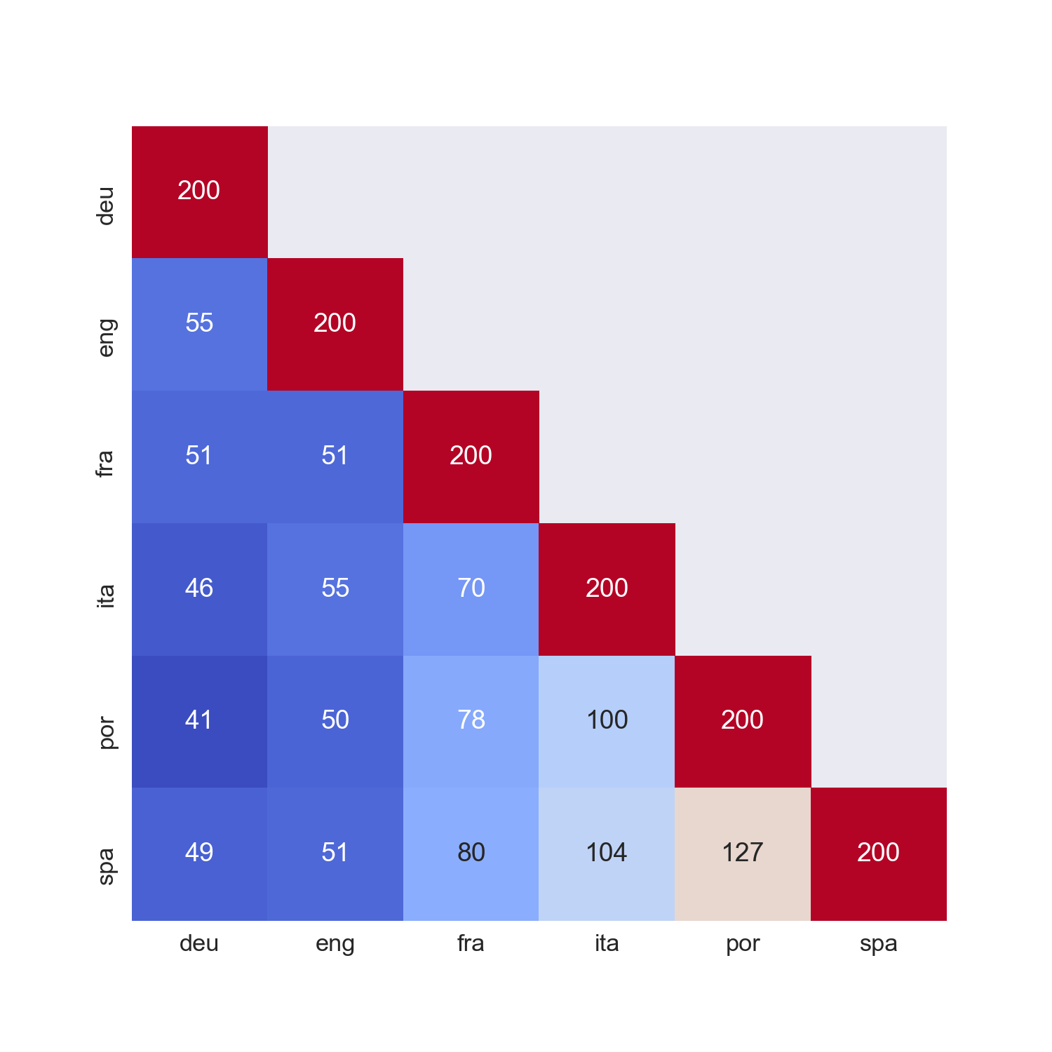
We now have the datasets in a form ready to be used to train our Neural Network. Before we do that, it would be useful to explore the dataset and build up a bit of an intuition around how well these features will do at predicting the languages. Figure 2 gives the number of trigrams each language has in common with the others. For example, English and German have 55 of their most common trigrams in common.
现在,我们已经准备好以训练我们的神经网络形式使用的数据集。 在此之前,对数据集进行探索并建立一些直觉,以了解这些功能在预测语言方面的表现会很有用。 图2给出了每种语言与其他语言共有的卦的数量。 例如,英语和德语有55个最常见的卦。
With 127, we see that Spanish and Portuguese have the most trigrams in common. This makes sense as, among all the languages, these two are the most lexically similar. What this means is that, using these features, our model may find it difficult to distinguish Spanish from Portuguese and visa versa. Similarly, Portuguese and German have the least trigrams in common and we could expect our model to be better at distinguishing these languages.
有了127,我们看到西班牙语和葡萄牙语具有最多的三字母组合。 这是有道理的,因为在所有语言中,这两种在词法上最相似。 这意味着使用这些功能,我们的模型可能会发现很难区分西班牙语和葡萄牙语,反之亦然。 同样,葡萄牙语和德语中的共有字母最少,我们可以期望我们的模型在区分这些语言方面更好。
造型 (Modelling)
We use the keras package to train our DNN. A softmax activation function is used in the model’s output layer. This means we have to transform our list of target variables into a list of one-hot encodings. This is done using the encode function below. This function takes a list of target variables and returns a list of one-hot encoded vectors. For example, [eng,por,por, fra,…] would become [[0,1,0,0,0,0],[0,0,0,0,1,0],[0,0,0,0,1,0],[0,0,1,0,0,0],…].
我们使用keras软件包来训练DNN。 在模型的输出层中使用softmax激活函数。 这意味着我们必须将目标变量列表转换为一键编码的列表。 使用下面的编码功能可以完成此操作。 此函数获取目标变量的列表,并返回一键编码矢量的列表。 例如,[eng,por,por,fra,...]将变为[[0,1,0,0,0,0],[0,0,0,0,1,0],[0,0, 0,0,1,0],[0,0,1,0,0,0],…]。
from sklearn.preprocessing import LabelEncoder
from keras.utils import np_utils


#Fit encoder
encoder = LabelEncoder()
encoder.fit(['deu', 'eng', 'fra', 'ita', 'por', 'spa'])


def encode(y):
    """
    Returns a list of one hot encodings
    Params
    ---------
        y: list of language labels
    """

    y_encoded = encoder.transform(y)
    y_dummy = np_utils.to_categorical(y_encoded)

    return y_dummy
Before choosing the final model structure, I did a bit of hyperparameter tuning. I varied the number of nodes in the hidden layers, the number of epochs and the batch-size. The hyperparameter combination that achieved the highest accuracy on the validation set was chosen for the final model.
在选择最终模型结构之前,我做了一些超参数调整。 我更改了隐藏层中的节点数,时期数和批处理大小。 选择在验证集上获得最高准确度的超参数组合作为最终模型。
The final model has 3 hidden layers with 500, 500 and 250 nodes respectfully. The output layer has 6 nodes, one for each language. The hidden layers all have ReLU activation functions and, as mentioned, the output layer has a softmax activation function. We train this model using 4 epochs and a batch size of 100. Using our training set and one-hot encoded target variable list, we train this DDN in the code below. In the end, we achieve a training accuracy of 99.70%.
最终模型具有3个隐藏层,分别具有500、500和250个节点。 输出层有6个节点,每种语言一个。 隐藏层均具有ReLU激活功能,并且如上所述,输出层具有softmax激活功能。 我们使用4个时期和100个批处理量训练该模型。使用我们的训练集和一个热编码的目标变量列表,我们在下面的代码中训练此DDN。 最终,我们达到了99.70%的训练精度。
from keras.models import Sequential
from keras.layers import Dense


#Get training data
x = train_feat.drop('lang',axis=1)
y = encode(train_feat['lang'])


#Define model
model = Sequential()
model.add(Dense(500, input_dim=663, activation='relu'))
model.add(Dense(500, activation='relu'))
model.add(Dense(250, activation='relu'))
model.add(Dense(6, activation='softmax'))
model.compile(loss='categorical_crossentropy', optimizer='adam', metrics=['accuracy'])


#Train model
model.fit(x, y, epochs=4, batch_size=100)
模型评估 (Model evaluation)
During the model training process, the model can become biased towards the training set as well as the validation set. So it is best to determine the model accuracy on an unseen test set. The final accuracy on the test set was 98.26%. This is lower than the training accuracy of 99.70% suggesting that some overfitting to the training set has occurred.
在模型训练过程中,模型可能会偏向训练集和验证集。 因此,最好在看不见的测试集中确定模型的准确性。 测试仪的最终精度为98.26%。 这低于99.70%的训练准确度,表明已对训练集过度拟合。
We can get a better idea of how well the model does for each language by looking at the confusion matrix in Figure 3. The red diagonal gives the number of correct predictions for each language. The off-diagonal numbers give the number of times a language was incorrectly predicted as another. For example, German is incorrectly predicted as English 10 times. We see that the model most often confuses either Portuguese for Spanish (124 times) or Spanish for Portuguese (61 times). This follows from what we saw when exploring our features.
通过查看图3中的混淆矩阵,我们可以更好地了解模型对每种语言的性能。红色对角线表示每种语言的正确预测数。 非对角线数字给出了一种语言被错误地预测为另一种语言的次数。 例如,德语被错误地预测为英语的10倍。 我们看到该模型最容易混淆葡萄牙语(西班牙语)(124次)或西班牙语(葡萄牙语)(61次)。 这是根据我们探索功能时看到的结果得出的。

The code used to create this confusion matrix is given below. Firstly, we use our model trained above to make predictions on the test set. Using these predicted languages and the actual languages, we create a confusion matrix and visualise it using a seaborn heatmap.
下面给出了用于创建此混淆矩阵的代码。 首先,我们使用上面训练的模型对测试集进行预测。 使用这些预测的语言和实际的语言,我们创建了一个混淆矩阵,并使用海洋热图对其进行了可视化。
import matplotlib.pyplot as plt
import seaborn as sns
from sklearn.metrics import accuracy_score,confusion_matrix


x_test = test_feat.drop('lang',axis=1)
y_test = test_feat['lang']


#Get predictions on test set
labels = model.predict_classes(x_test)
predictions = encoder.inverse_transform(labels)


#Accuracy on test set
accuracy = accuracy_score(y_test,predictions)
print(accuracy)


#Create confusion matrix
lang = ['deu', 'eng', 'fra', 'ita', 'por', 'spa']
conf_matrix = confusion_matrix(y_test,predictions)
conf_matrix_df = pd.DataFrame(conf_matrix,columns=lang,index=lang)


#Plot confusion matrix heatmap
plt.figure(figsize=(10, 10), facecolor='w', edgecolor='k')
sns.set(font_scale=1.5)
sns.heatmap(conf_matrix_df,cmap='coolwarm',annot=True,fmt='.5g',cbar=False)
plt.xlabel('Predicted',fontsize=22)
plt.ylabel('Actual',fontsize=22)
In the end, the test accuracy of 98.26% leaves room for improvement. In terms of feature selection, we have kept things simple and have just selected the 200 most common trigrams for each language. A more complicated approach could help us differentiate the languages that are more similar. For example, we could select trigrams that are common in Spanish but not so common in Portuguese and visa versa. We could also experiment with different models. Hopefully, this is a good starting point for your language identification experiments.
最后,测试精度为98.26%,尚有待改进。 在功能选择方面,我们使事情保持简单,并为每种语言选择了200个最常见的三字母组。 一种更复杂的方法可以帮助我们区分更相似的语言。 例如,我们可以选择在西班牙语中很常见但在葡萄牙语中却不太常见的三字组,反之亦然。 我们也可以尝试不同的模型。 希望这是您进行语言识别实验的良好起点。
图片来源 (Image Sources)
All images are my own or obtain from www.flaticon.com. In the case of the latter, I have a “Full license” as defined under their Premium Plan.
所有图像都是我自己的,或从www.flaticon.com获得。 对于后者,我拥有其“ 高级版计划 ”中定义的“完整许可证”。
翻译自: https://towardsdatascience.com/deep-neural-network-language-identification-ae1c158f6a7d
浅层神经网络 深层神经网络


 2553
2553


 被折叠的 条评论
为什么被折叠?
被折叠的 条评论
为什么被折叠?
 到【灌水乐园】发言


