


神经网络解决机器学习预测
The dataset and code for this project is available in my GitHub repository. The link for the same is shared at the end of this story.
我的GitHub存储库中提供了该项目的数据集和代码。 故事的结尾共享了相同的链接。
The cybercrime industry has been gaining traction over the years, especially owing to the fact that more and more data (personal and organizational) is available on digital mediums. Today, the issues posed by cybercrime cause companies to bleed millions of dollars across the globe. In a study conducted across 507 organizations in 16 countries and regions across 17 industries by the Ponemon Institute, it was defined that the global average cost of data breach for 2019 stands at $3.92 Million, a 1.5% increase from the 2018 estimate. Organizations worldwide are heavily investing into the capabilities of predictive analytics using machine learning and artificial intelligence to mitigate these challenges.
吨他网络犯罪行业已获得牵引力,多年来,尤其是因为这样的事实:越来越多的数据(个人和组织)提供数字媒体。 如今,网络犯罪带来的问题使公司在全球范围内流失了数百万美元。 Ponemon Institute在16个国家和地区的17个行业中的507个组织中进行的一项研究确定,2019年全球数据泄露的平均成本为392万美元,比2018年的估计增加1.5%。 全世界的组织都在大力投资使用机器学习和人工智能来缓解这些挑战的预测分析功能。
As per a report by Capgemini Research Institute (2019), 48% of organizations say that their budget for implementation of predictive analytics in cybersecurity will increase by 29% in the fiscal year 2020. 56% of senior executives say that cybersecurity analysts are overworked and close to a quarter of them are not able to successfully investigate all identified issues. 64% of organizations say that predictive analytics lowers the cost of threat detection and response and reduces the overall detection time by up to 12%.
根据Capgemini研究院(2019)的报告 ,48%的组织表示其在网络安全方面实施预测分析的预算将在2020财年增加29%.56%的高级管理人员表示,网络安全分析师工作过度且他们中有将近四分之一无法成功调查所有已发现的问题。 64%的组织表示,预测分析可降低威胁检测和响应的成本,并将总体检测时间减少多达12%。
Considering the above, the application of predictive analytics into investigating the endpoints which are likely to be infected by malware becomes imperative for organizations in the long run. The study explores this objective, using the knowledge of the specifications of certain hardware and software aspects of an organization’s endpoint (Desktops, Laptops, Mobiles, Servers, etc.).
考虑到上述情况,从长远来看,将预测性分析应用于调查可能被恶意软件感染的端点对于组织而言势在必行。 该研究使用组织端点(台式机,便携式计算机,移动设备,服务器等)的某些硬件和软件方面的规范知识来探索此目标。
The data has a mixture of both categorical and numerical variables. In this study, one of the primary challenges faced was the presence of a large percentage of missing data in the dataset. The data upon further analysis was categorized as Missing at Random (MAR). The variables in the dataset are:
数据混合了类别变量和数值变量。 在这项研究中,面临的主要挑战之一是数据集中大量丢失数据的存在。 经过进一步分析的数据被归类为随机缺失(MAR)。 数据集中的变量为:

缺失数据分类和多重插补技术 (Missing Data Classification & Multiple Imputation Technique)
Missing data or missing values is nothing but the absence of data value in a variable of interest for the study being performed. It brings about several issues while performing statistical analysis.
数据丢失或值丢失不过是正在进行的研究感兴趣的变量中没有数据值而已。 进行统计分析时会带来一些问题。

Most statistical analysis methods reject the missing values, thus reducing the size of the dataset to work with. Often, having not enough data to work with creates models that produces results which are statistically not significant. Also, missing data might lead to cases where the results are misleading. Results are often biased towards certain segment/segments that are overrepresented in the population.
大多数统计分析方法都拒绝缺失值 ,从而减小了要使用的数据集的大小。 通常, 没有足够的数据可用于创建模型,这些模型产生的结果在统计上并不重要 。 另外,数据丢失可能会导致结果产生误导。 结果通常会偏向总体中代表过多的某些细分市场。
缺少数据分类 (Missing Data Classification)
The classification of missing data was first discussed by Rubin in his paper titled ‘Inference and Missing Data’. According to his theory, every data point in a dataset has some probability of being missing. Based on this probability, Rubin classifies missing data into the following types:
鲁宾(Rubin)在他的题为“ 推理和丢失数据 ”的论文中首先讨论了丢失数据 的分类 。 根据他的理论,数据集中的每个数据点都有丢失的可能性。 基于此概率,Rubin将丢失的数据分为以下几种类型:
Missing Completely at Random (MCAR): The missingness of data, in this case, is not related to the other responses or information in the data in anyway. The probability of any data point being missing in the dataset remains equal for all the other data points. In simpler words, there is no identifiable pattern in the missingness of the data. An important thing to be noticed when dealing with MCAR is that analysis done on MCAR produces unbiased results.
完全随机丢失(MCAR) :在这种情况下,数据的丢失无论如何都与数据中的其他响应或信息无关。 对于所有其他数据点,数据集中丢失任何数据点的可能性仍然相等。 用简单的话来说,数据的缺失没有可识别的模式。 处理MCAR时要注意的重要一点是,对MCAR进行的分析会产生无偏见的结果。
Missing at Random (MAR): MAR is a wider classification of missing data when compared to MCAR, and in some terms more realistic too. In the case of MAR, the probability of the missingness of data is similar for certain subsets of the data defined for the statistical study. The missingness of the data can be attributed to the other data that is present and hence can be predicted. Again, in simpler words, in case of MAR, there is a pattern to the missingness of the data.
随机缺失(MAR) :与MCAR相比,MAR是对缺失数据的更广泛分类,从某种意义上说也更现实。 对于MAR,对于为统计研究定义的某些数据子集,数据丢失的可能性相似。 数据的缺失可以归因于存在的其他数据,因此可以被预测。 再次,换句话说,对于MAR,存在数据丢失的模式。
Not Missing at Random (NMAR): Data which is not classified as MCAR and MAR is classified as NMAR.
随机不丢失(NMAR) :未分类为MCAR和MAR的数据分类为NMAR。
使用MICE的多重插补(通过链式方程进行的多元插补) (Multiple Imputation using MICE (Multivariate Imputation via Chained Equations))
Multiple Imputation method for estimating missing data was proposed by Rubin (1987). The method starts with a dataset that contains missing values and then goes on to create several sets of imputed values for the missing data using a statistical model like linear regression. This is followed by calculating the parameters of interest for each of the imputed data set, which are finally pooled together into one estimate. Figure below shows a pictorial representation of a Multiple Imputation method of the 4th order.
Rubin(1987)提出了用于估计缺失数据的多重插补方法。 该方法从包含缺失值的数据集开始,然后继续使用线性回归之类的统计模型为缺失数据创建多组估算值。 接下来,为每个估算数据集计算感兴趣的参数,最后将这些参数汇总到一个估计中。 下图显示了四阶多重插补方法的图形表示。

Single imputation methods like Mean Imputation, Regression Imputation, etc. work on the assumption that the estimated imputed value is the true value, neglecting the uncertainties related to the prediction of the imputed value.
单一插补方法(例如均值插补,回归插补等)在假定估算的插补值是真实值的假设下工作,而忽略了与插补值的预测有关的不确定性。
The advantages of using multiple imputation over single imputation are:
使用多重插补优于单一插补的优点是:
- The standard error which was too small in case of single imputation techniques is mitigated well by using multiple imputation. 通过使用多次插补,可以很好地减轻单次插补技术下的标准误差。
- Multiple imputation performs well not only with MCAR data but also with MAR data. 多重插补不仅适用于MCAR数据,而且适用于MAR数据。
- The variation in data that is received across the multiple imputed dataset helps in offsetting any sort of bias. This is achieved by adding the uncertainties that were missing as part of the single imputation techniques. This in turn increases the precision and results in robust statistics which leads to better analysis that might be performed on the data. 跨多个估算数据集接收的数据变化有助于抵消任何类型的偏差。 这是通过添加作为单一归因技术的一部分而缺少的不确定性来实现的。 反过来,这会提高精度并产生可靠的统计信息,从而可以对数据进行更好的分析。
One of the most popular methods of performing multiple imputation in R is using the MICE (Multivariate Imputation via Chained Equations) package. The code for the implementation of MICE on our dataset is shared below:
在R中执行多重插补的最流行的方法之一是使用MICE(通过链式方程进行多元插补)程序包。 在我们的数据集上实现MICE的代码在以下共享:
library(mice)
library(caret)df = read.csv('Data.csv')
View(df)#checking for NAs in the data
sapply(df, function(x) sum(is.na(x)))##############converting into factors(categorical variables)
df$HasTpm = as.factor(df$HasTpm)
df$IsProtected = as.factor(df$IsProtected)
df$Firewall = as.factor(df$Firewall)
df$AdminApprovalMode = as.factor(df$AdminApprovalMode)
df$HasOpticalDiskDrive = as.factor(df$HasOpticalDiskDrive)
df$IsSecureBootEnabled = as.factor(df$IsSecureBootEnabled)
df$IsPenCapable = as.factor(df$IsPenCapable)
df$IsAlwaysOnAlwaysConnectedCapable = as.factor(df$IsAlwaysOnAlwaysConnectedCapable)
df$IsGamer = as.factor(df$IsGamer)
df$IsInfected = as.factor(df$IsInfected)str(df)
ncol(df)###############REMOVING MachineId FROM DATA FRAME
df = df[,-c(1)]##############IMPUTATION OF MISSING DATA USING MICE
init = mice(df, maxit=0)
meth = init$method
predM = init$predictorMatrix#Excluding the output column IsInfected as a predictor for Imputation
predM[, c("IsInfected")]=0#Excluding these variables from imputation as they don't have null valuesmeth[c("ProductName","HasTpm","Platform","Processor","SkuEdition","DeviceType","HasOpticalDiskDrive","IsPenCapable","IsInfected")]=""#Specifying the imputation methods for the variables with missing data

meth[c("SystemVolumeTotalCapacity","PrimaryDiskTotalCapacity","TotalPhysicalRAM")]="cart" meth[c("Firewall","IsProtected","IsAlwaysOnAlwaysConnectedCapable","AdminApprovalMode","IsSecureBootEnabled","IsGamer")]="logreg" meth[c("PrimaryDiskTypeName","AutoUpdate","GenuineStateOS")]="polyreg"#Setting Seed for reproducibility
set.seed(103)#Imputing the data
class(imputed)
imputed = mice(df, method=meth, predictorMatrix=predM, m=5)
imputed <- complete(imputed)sapply(imputed, function(x) sum(is.na(x)))sum(is.na(imputed))
合奏学习方法 (Ensemble Learning Methods)
Ensemble learning methods use the combined computational power of multiple models to classify and solve the problem at hand. When compared to ordinary learning algorithms that create only one learning model, ensemble learning methods create multiple such models and combine them to make the final model that makes more efficient classifications. Ensemble learning is also called as committee-based learning or learning multiple classifier systems.
集成学习方法使用多个模型的组合计算能力来分类和解决当前的问题。 与仅创建一个学习模型的普通学习算法相比,集成学习方法会创建多个这样的模型,并将它们组合起来以构成最终模型,从而使分类更为有效 。 集成学习也称为基于委员会的学习或学习多个分类器系统。
Ensemble learning methods are used and appreciated because of their ability to boost the performance of weak learners, often known as base learners. This in turn produces predictions with higher accuracy and stronger generalization performance. The models created also are more robust in nature and respond well to noise in data.
集成学习方法之所以得到使用和赞赏,是因为它们能够提高弱学习者 (通常被称为基础学习者)的表现。 反过来,这将产生具有更高准确性和更强泛化性能的预测 。 创建的模型本质上也更健壮,并且对数据噪声响应良好。
套袋合奏学习 (Bagging Ensemble Learning)
Bagging is an acronym for Bootstrap Aggregating and is used to solve both classification and regression problems. The method of Bagging involves creating multiple samples which are random in nature with replacement. These samples are used to create models, the results from which are amalgamated together. The advantage of using Bagging algorithms lies in the fact that they reduce the chances of a predictive model overfitting the data. Since every model is built on a different set of data, the variance error component of the reducible error in the model is low, which means that the model handles the variance in test data well.For this study, we use two bagging algorithms, the Bagged CART Algorithm and the Random Forest Algorithm.
Bagging是Bootstrap Aggregation的首字母缩写,用于解决分类和回归问题。 套袋的方法涉及创建多个样本,这些样本本质上是随机的,并且需要替换。 这些样本用于创建模型,将其结果合并在一起。 使用Bagging算法的优势在于,它们减少了预测模型过度拟合数据的机会。 由于每个模型都基于不同的数据集,因此模型中可减少误差的方差误差分量很低,这意味着该模型可以很好地处理测试数据中的方差。 在本研究中,我们使用两种装袋算法,即袋装CART算法和随机森林算法。

促进整体学习 (Boosting Ensemble Learning)
Boosting ensemble learning works on an iterative approach of adjusting weights of an observation present in the training dataset based upon the performance of the previous classification model. The weight for an observation is increased if it is classified incorrectly and decreased if classified correctly. Boosting ensemble learning has it’s in advantage in cases where the bias error component of reducible error is high. Boosting decreases this bias error and helps in building stronger predictive models.For this study, we use two bagging algorithms, the C5.0 Decision Trees Boosting Algorithm & Stochastic Grading Boosting Algorithm.
促进整体学习的方法是基于先前分类模型的性能,通过迭代方法调整训练数据集中存在的观测值的权重。 如果分类不正确,则观察权重增加;如果分类正确,则权重降低。 在可减少误差的偏倚误差成分较高的情况下,促进整体学习具有优势。 提升可减少此偏差误差,并有助于建立更强大的预测模型。 在本研究中,我们使用两种装袋算法:C5.0决策树增强算法和随机分级增强算法。

The R code for the various models used is given below:
下面给出了所使用的各种模型的R代码:
# Example of Boosting Algorithms
control <- trainControl(method="repeatedcv", number=10, repeats=3, classProbs = TRUE, summaryFunction = twoClassSummary)
seed <- 7
metric <- "ROC"# C5.0
set.seed(seed)
fit.c50 <- train(IsInfected~., data=imputed, method="C5.0", metric=metric, trControl=control)# Stochastic Gradient Boosting
set.seed(seed)
fit.gbm <- train(IsInfected~., data=imputed, method="gbm", metric=metric, trControl=control, verbose=FALSE)# summarize results
boosting_results <- resamples(list(c5.0=fit.c50, gbm=fit.gbm))
summary(boosting_results)
dotplot(boosting_results)# Example of Bagging algorithmscontrol <- trainControl(method="repeatedcv", number=10, repeats=3, classProbs = TRUE, summaryFunction = twoClassSummary)seed <- 7metric <- "ROC"# Bagged CART
set.seed(seed)
fit.treebag <- train(IsInfected~., data=imputed, method="treebag", metric=metric, trControl=control)# Random Forest
set.seed(seed)
fit.rf <- train(IsInfected~., data=imputed, method="rf", metric=metric, trControl=control)# summarize results
bagging_results <- resamples(list(treebag=fit.treebag, rf=fit.rf))
summary(bagging_results)
dotplot(bagging_results)
结果 (The Results)
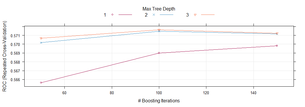
After applying various ensemble models, it is found that the Stochastic Gradient Boosting model with a tree depth of 3 and number of trees as 100 gives the best values of accuracy and the Area Under the ROC curve.
在应用各种集成模型后,发现树深度为3且树数为100的随机梯度增强模型给出了精度和ROC曲线下面积的最佳值。

The study works towards establishing the hypothesis that with the correct knowledge of the specifications of organizational endpoints (both software and hardware), it is possible to predict the likeliness of an endpoint to get infected by malware attacks and other cybersecurity threats. In order to achieve the aim of this study, several real-life challenges related to data were faced, like understanding missing data, the imputation of missing data using multiple imputation technique, challenges with cross validation of data and performance evaluation of the models.
这项研究旨在建立一种假设,即只要正确了解组织端点的规范 (包括软件和硬件), 就可以预测端点被恶意软件攻击和其他网络安全威胁感染的可能性。 为了达到本研究的目的,面临着与数据相关的一些现实挑战,例如理解缺失数据,使用多重插补技术对缺失数据进行插补,数据交叉验证和模型性能评估等挑战。
The list of variables used in the study for building the model is not exhaustive in nature, several new metrics and variables can be added based upon the availability and applicability with respect to various organizations to build more accurate and robust models.
研究中用于构建模型的变量列表本质上并不详尽,可以根据各种组织的可用性和适用性来添加几个新的指标和变量,以构建更准确,更可靠的模型。
神经网络解决机器学习预测


 1万+
1万+

 被折叠的 条评论
为什么被折叠?
被折叠的 条评论
为什么被折叠?
 到【灌水乐园】发言


