tensorflow入门_TensorFlow终极入门指南

tensorflow入门

介绍 (Introduction)

In this tutorial, we will cover TensorFlow in enough depth so that you can train machine learning models from scratch!

在本教程中，我们将足够深入地介绍TensorFlow，以便您可以从头开始训练机器学习模型！

TensorFlow is Google’s flagship library for machine learning development. It is used both commercially and by developers for building and deploying machine learning modules. There are two broad versions of TensorFlow — 2.X and 1.X. Both allow for similar functionality, but 2.X uses a cleaner API and has some slight upgrades. It is important to understand that TensorFlow has grown from just a software library to an entire ecosystem for all types of machine learning. APIs like Keras make it extremely simple to train and test deep learning networks in a few lines. (We will cover this towards the end of this tutorial). This tutorial assumes a basic understanding of Python 3 and some degree of familiarity with linear algebra.

TensorFlow是Google的机器学习开发旗舰库。 商业和开发人员都可以使用它来构建和部署机器学习模块。 TensorFlow有两种广泛的版本-2.X和1.X。 两者都允许类似的功能，但是2.X使用更简洁的API并进行了一些轻微的升级。 重要的是要理解TensorFlow已经从一个软件库发展到了适用于所有类型机器学习的整个生态系统。 像Keras这样的API使得在几行中训练和测试深度学习网络变得极其简单。 (我们将在本教程结束时对此进行介绍)。 本教程假定您对Python 3有基本的了解，并且对线性代数有一定程度的了解。

数学背景 (Mathematical Background)

Let’s get started with some fundamental background on the mathematics behind TensorFlow. There are three main constructs for TensorFlow operations: vectors, arrays (matrices), tensors. A vector is a mathematical object that has a direction and a magnitude. It is used to find the position of one point in space relative to another point. An array is an arrangement or a series of elements such as symbols, numbers, or expressions. Arrays can be n-dimensional, so a matrix is an array with 2 dimensions. A tensor is an object describing the linear relationship among scalars, vectors, and other tensors. In other words, it is the stacking of multiple arrays to create higher dimensional structures. A practical example of a tensor in action is with an image. When an RGB image is processed, it is a 3-D tensor with layers for each color across the dimensions of height and width. Hopefully, this graphic should clarify the differences:

让我们从TensorFlow背后的数学基础知识入手。 TensorFlow操作有三种主要构造：向量，数组(矩阵)，张量。 向量是具有方向和大小的数学对象。 它用于查找空间中一个点相对于另一点的位置。 数组是排列或一系列元素，例如符号，数字或表达式。 数组可以是n维的，因此矩阵是2维的数组。 张量是描述标量，向量和其他张量之间线性关系的对象。 换句话说，它是多个阵列的堆叠以创建更高维的结构。 张量的实际例子是图像。 处理RGB图像时，它是一个3-D张量，其中每种颜色的层在高度和宽度的整个维度上都有层。 希望此图可以澄清差异：

Source 资源

It would also be useful to understand the Rank of a Matrix. The rank of a Matrix is the number of linearly independent column or row vectors. Before moving on, we will assume that you understand basic linear algebra — transposes, inverses, matrix multiplication, etc. Let’s now define these concepts with some code.

了解矩阵的等级也将很有用。 矩阵的秩是线性独立的列或行向量的数量。 在继续之前，我们假设您了解基本的线性代数-转置，逆，矩阵乘法等。现在让我们用一些代码定义这些概念。

import numpy as np a = np.array([[1,2,3], [4,5,6], np.int16)
b = np.mat([1,2,3])

With this code, we use the NumPy library to initialize both a numpy.matrix and a 2D numpy.ndarrray. There are basic differences in these two structures, for example, the fact that numpy.matrix has a proper matrix multiplication interface, but they effectively achieve a very similar purpose. Let’s now discuss how we can implement a tensor. Remember that a tensor is an object that describes the linear relationship between scalars, vectors, and other tensors. A 0th order tensor (or Rank 0) can be represented by a scalar. A 1st order tensor (or Rank 1) can be represented by an array (1-d vector). A 2nd order tensor (or Rank 2) can be represented by a matrix (2-d array). A 3rd order tensor (or Rank 3) is a 3-dimensional array. These examples are implemented in code for reference.

通过此代码，我们使用NumPy库初始化numpy.matrix和2D numpy.ndarrray。 这两种结构存在基本差异，例如numpy.matrix具有适当的矩阵乘法接口这一事实，但它们实际上达到了非常相似的目的。 现在让我们讨论如何实现张量。 请记住，张量是描述标量，向量和其他张量之间线性关系的对象。 0阶张量(或等级0)可以用标量表示。 一阶张量(或等级1)可以由数组(1-d向量)表示。 二阶张量(或等级2)可以由矩阵(二维数组)表示。 3阶张量(或等级3)是3维数组。 这些示例以代码形式实现以供参考。

t_0 = np.array(50, dtype=np.int32)t_1 = np.array([b"apple", b"peach", b"grape"])t_2 = np.array([[True, False, False], [False, False, True]])t_3 = np.array([[ [0,0], [0,1], [0,2] ], [ [0,0], [0,1], [0,2] ],[ [0,0], [0,1], [0,2] ]])

Objects in TensorFlow will always have a shape. A shape describes the number of dimensions a tensor can hold, including the length of each dimension. The shape of TensorFlow can be either a list or a tuple. This may not be simple to understand at first, so let’s break it down with an example. What would the shape be for the list [2,3]? This list describes the shape of a 2-D tensor of length 2 in its first dimension and length 3 in its second dimension. In other words, this is a 2x3 matrix! Let’s see some more shapes broken done in code:

TensorFlow中的对象将始终具有形状。 形状描述张量可以容纳的维数，包括每个维的长度。 TensorFlow的形状可以是列表或元组。 乍一看，这可能并不容易理解，所以让我们用一个例子来分解它。 列表[2,3]的形状是什么？ 该列表描述了一个二维张量的形状，该二维张量在其第一维度上的长度为2，在其第二维度上的长度为3。 换句话说，这是2x3矩阵！ 让我们来看一些在代码中完成的形状分解：

s_1_flex = [None]s_2_flex = (None, 3)s_3_flex = [2, None, None]s_any = None

If you are confused about what the “None” keyword refers to, it says that the dimension can be of any size. For example, s_1_flex is a 1-D array with a size of N.

如果您对“ None”关键字的含义感到困惑，则说明该尺寸可以是任意大小。 例如， s_1_flex是大小为N的一维数组。

TensorFlow中的图形和会话 (Graphs and Sessions in TensorFlow)

At the center of Tensorflow is the concept of the graph. Before we discuss the graph, let’s talk about eager execution. Eager execution in TensorFlow means that each operation is executed by Python, operation by operation. Eager TensorFlow runs on GPUs and is easy to debug. For some of us, we will be happy to keep our TensorFlow projects in Python and will never leave. However, for other users, eager execution means prevents a “host of accelerations otherwise available” [1]. Luckily, there are ways to both enable and disable eager execution:

Tensorflow的中心是图形的概念。 在讨论图之前，让我们谈谈热切的执行。 TensorFlow中急切的执行意味着每个操作都由Python执行，一个接一个地执行。 Eager TensorFlow在GPU上运行，易于调试。 对于我们中的某些人，我们很乐意将TensorFlow项目保留在Python中，并且永远不会离开。 但是，对于其他用户而言，急切的执行手段可以防止“否则将有大量的加速” [1]。 幸运的是，有一些方法可以启用和禁用急切执行：

import tensorflow as tf# to check for eager execution
tf.executing_eagerly()
# to enable eager execution
tf.compat.v1.enable_eager_execution()
# to disable eager execution
tf.compat.v1.disable_eager_execution()
# After eager execution is enabled, operations are executed as they are defined and Tensor objects hold concrete values, which can be accessed as numpy.ndarray`s through the numpy() method.assert tf.multiply(6, 7).numpy() == 42

If we want to extract our operations so that we can access them outside of Python, we can make them into a graph. As a note, TensorFlow is updated rapidly and functions and definitions may be adjusted, so always check what version of TensorFlow you are using. This can be done in the following line of code:

如果我们要提取操作以便可以在Python之外访问它们，则可以将它们制成图形。 请注意，TensorFlow会快速更新，功能和定义可能会有所调整，因此请始终检查您所使用的TensorFlow版本。 这可以在下面的代码行中完成：

print(tf.__version__)

For this tutorial, we are using Tensorflow 2.3. Now back to graphs! Graphs are data structures that contain a set of tf.Operation objects. Graphs are useful since they can be saved, run, and restored without the original Python code. A TensorFlow graph is a specific type of directed graph that is used for defining computational structure. In TensorFlow graphs, there are three main objects which can be employed for operations. First is the constant. This creates a node that takes a value and does not change. Here is an example of a constant in action: tf.constant(6,tf.int32,name=’A'). The next graph object in TensorFlow is the variable. Variables are stateful nodes that output their current value; meaning that they can retain their value over multiple executions of a graph. Here is an example of a variable in action: w = tf.Variable(, name=). The final object is the placeholder. Placeholders can feed in future values at runtime in a graph. There are used when a graph depends on external data. Here is one implemented: tf.compat.v1.placeholder(tf.int32, shape=[3], name='B'). Let’s now launch our first graph. This example does not explicitly launch a graph, but it shows how we can run operations within a Session:

在本教程中，我们使用Tensorflow 2.3。 现在回到图表！ 图是tf.Operation对象的数据结构。 图非常有用，因为它们可以在没有原始Python代码的情况下进行保存，运行和还原。 TensorFlow图是一种特定类型的有向图，用于定义计算结构。 在TensorFlow图中，可以使用三个主要对象进行操作。 首先是常数 。 这将创建一个带值且不会更改的节点。 这是一个作用中的常量的示例： tf.constant(6,tf.int32,name='A') 。 TensorFlow中的下一个图形对象是变量。 变量是输出其当前值的有状态节点。 表示他们可以在多次执行图形时保留其值。 这是一个作用中的变量的示例： w = tf.Variable(, name=) 。 最后一个对象是占位符 。 占位符可以在运行时在图形中提供将来的值。 当图形依赖于外部数据时使用。 这是一个实现的方法： tf.compat.v1.placeholder(tf.int32, shape=[3], name='B') 。 现在启动第一个图形。 此示例未明确启动图，但显示了如何在Session中运行操作：

# Launch the graph in a session.with tf.compat.v1.Session() as sess:   # input nodes
   a = tf.constant(5, name="input_a")
   b = tf.constant(3, name="input_b")   # next two nodes
   c = tf.math.multiply(a, b, name="input_c")
   d = tf.math.add(a, b, name="input_d")   # final node
   e = tf.add(c, d, name="input_e")   print(sess.run(e))

To add nodes to our “graph”, we can add, subtract, or multiply existing nodes. In the case above, nodes c, d, and e are all operations of previously initialized nodes. To run this graph, we ran it in what is known as a tf.Session. When not using eager execution, we will need to run our graph in a Session. In this case, we ran it in a Session known as sess. In general, sessions allow us to execute graphs. In TensorFlow 2, sessions are essentially gone. Everything is run in one global runtime. However, for the purposes of this tutorial, we will continue to review Sessions. Here is an example of a concrete graph in action:

要将节点添加到“图形”中，我们可以添加，减去或乘以现有节点。 在上述情况下，节点c，d和e均为先前初始化的节点的操作。 要运行此图，我们在称为tf.Session运行它。 当不使用急切执行时，我们将需要在Session中运行图形。 在这种情况下，我们在称为sess的会话中运行了它。 通常，会话允许我们执行图。 在TensorFlow 2中，会话基本上消失了。 一切都在一个全局运行时中运行。 但是，出于本教程的目的，我们将继续审查会议。 这是一个具体的图表示例：

graph = tf.Graph()
with graph.as_default():
  variable = tf.Variable(42, name='foo')
  initialize = tf.global_variables_initializer()
  assign = variable.assign(13)with tf.Session(graph=graph) as sess:
  sess.run(initialize)
  sess.run(assign)
  print(sess.run(variable))
# Output: 13

In this code, we create a graph and initialize a variable named “foo”. We then assign “foo” to a new value. After creating the graph, we run it in a Session. Let’s clarify. Graphs and sessions are not necessary if eager execution is enabled. In other words, there would be no need for sess.run().

在此代码中，我们创建一个图形并初始化一个名为“ foo”的变量。 然后，我们将“ foo”分配给新值。 创建图后，我们在会话中运行它。 让我们澄清一下。 如果启用了急切执行，则不需要图形和会话。 换句话说，不需要sess.run() 。

张量板 (Tensorboard)

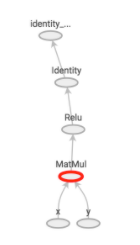
Now that we have discussed how graphs and sessions work in practice, you must be wondering — how do we examine them? We can use a tool known as Tensorboard. This is a tool integrated with Tensorflow 2.0 and it can be used to visualize the graph. It also has other tools to understand, debug, and optimize the model. The backend is now tf.keras in TensorFlow 2.0. Let’s now use Tensorboard to visualize a graph. Here is a simple starting example. Note that you can test this code out in Google Colab:

既然我们已经讨论了图形和会话在实践中是如何工作的，那么您一定想知道-我们如何检查它们？ 我们可以使用称为Tensorboard的工具。 这是与Tensorflow 2.0集成的工具，可用于可视化图形。 它还具有其他工具来理解，调试和优化模型。 后端现在是TensorFlow 2.0中的tf.keras。 现在让我们使用Tensorboard可视化图形。 这是一个简单的开始示例。 请注意，您可以在Google Colab中测试此代码：

%load_ext tensorboardsummary_writer = tf.summary.create_file_writer('logs/summaries')with summary_writer.as_default():
  tf.summary.scalar('scalar', 3.5, step=2)tensorboard --logdir /logs/summaries

This is a simple example where we write a tf scalar to our summary writer. We then run it in logs/summaries (our directory) to access Tensorboard. In most cases, Tensorboard output usually looks something like this:

这是一个简单的示例，其中我们向摘要编写器编写了tf标量。 然后，我们在logs/summaries (我们的目录)中运行它以访问Tensorboard。 在大多数情况下，Tensorboard输出通常如下所示：

Graph Output

图形输出

Let’s now unpack a more sophisticated example of using Tensorboard to visualize and debug graphs:

现在让我们打开一个使用Tensorboard可视化和调试图形的更复杂的示例：

# Load the TensorBoard notebook extension
%load_ext tensorboardimport tensorflow as tf
import datetime# Clear any logs from previous runs
!rm -rf ./logs/# initialize your directory 
logdir = INSERT_DIRECTORYg = tf.compat.v1.Graph()with g.as_default():
  step = tf.Variable(0, dtype=tf.int64)
  step_update = step.assign_add(1)
  writer = tf.summary.create_file_writer(logdir)
  with writer.as_default():
    tf.summary.scalar("my_metric", 0.5, step=step)
all_summary_ops = tf.compat.v1.summary.all_v2_summary_ops()
writer_flush = writer.flush()with tf.compat.v1.Session(graph=g) as sess:
  sess.run([writer.init(), step.initializer])  for i in range(100):
    sess.run(all_summary_ops)
    sess.run(step_update)
    sess.run(writer_flush)# run in tensorboard
%tensorboard --logdir logdir

This example uses the tf.summary.create_file_writer(logdir) to make sure that the output is read in Tensorboard. Now that we have seen Tensorboard in action, we’ve finished the core concepts of TensorFlow. However, TensorFlow is not as useful if we do not apply it for machine learning. We will now walk through Keras, TensorFlow’s simple API for training neural networks.

本示例使用tf.summary.create_file_writer(logdir)来确保在Tensorboard中读取了输出。 现在我们已经看到了Tensorboard的实际作用，我们已经完成了TensorFlow的核心概念。 但是，如果我们不将TensorFlow应用于机器学习，它就不会有用。 我们现在将逐步介绍TensorFlow用于训练神经网络的简单API Keras。

凯拉斯 (Keras)

Simply put, Keras makes it quite simple to train and test your machine learning models. Let’s now demonstrate Keras in action. (All Credit to TensorFlow) We start by importing libraries and checking our version. (This tutorial uses Tf 2.3):

简而言之，Keras使训练和测试您的机器学习模型变得非常简单。 现在让我们演示Keras的动作。 ( 全部 归功于TensorFlow )我们首先导入库并检查我们的版本。 (本教程使用Tf 2.3)：

# TensorFlow and tf.keras
import tensorflow as tf
from tensorflow import keras
# Helper libraries
import numpy as np
import matplotlib.pyplot as plt
print(tf.__version__)

Let’s now download a sample dataset. In this case, we will use the Fashion MNIST Dataset. The code below downloads the set directly from keras.datasets:

现在让我们下载一个样本数据集。 在这种情况下，我们将使用Fashion MNIST数据集。 以下代码直接从keras.datasets下载集合：

fashion_mnist = keras.datasets.fashion_mnist
(train_images, train_labels), (test_images, test_labels) = fashion_mnist.load_data()

When we load this dataset, we get four NumPy arrays: train_images, train_labels, test_images, test_labels. If you are familiar with machine learning then you would know that we need a certain number of images (data) to train and some samples to test on. Each image in our dataset is a 28x28 NumPy Array and the pixel values range from 0 to 255. The labels are an array of integers, ranging from 0 to 9. These correspond to the following:

加载此数据集时，我们得到四个NumPy数组：train_images，train_labels，test_images，test_labels。 如果您熟悉机器学习，那么您会知道我们需要训练一定数量的图像(数据)和一些样本进行测试。 我们的数据集中的每个图像都是一个28x28 NumPy数组，像素值的范围是0到255。标签是一个整数数组，范围是0到9。它们对应于以下内容：

Labels for each class

每个班级的标签

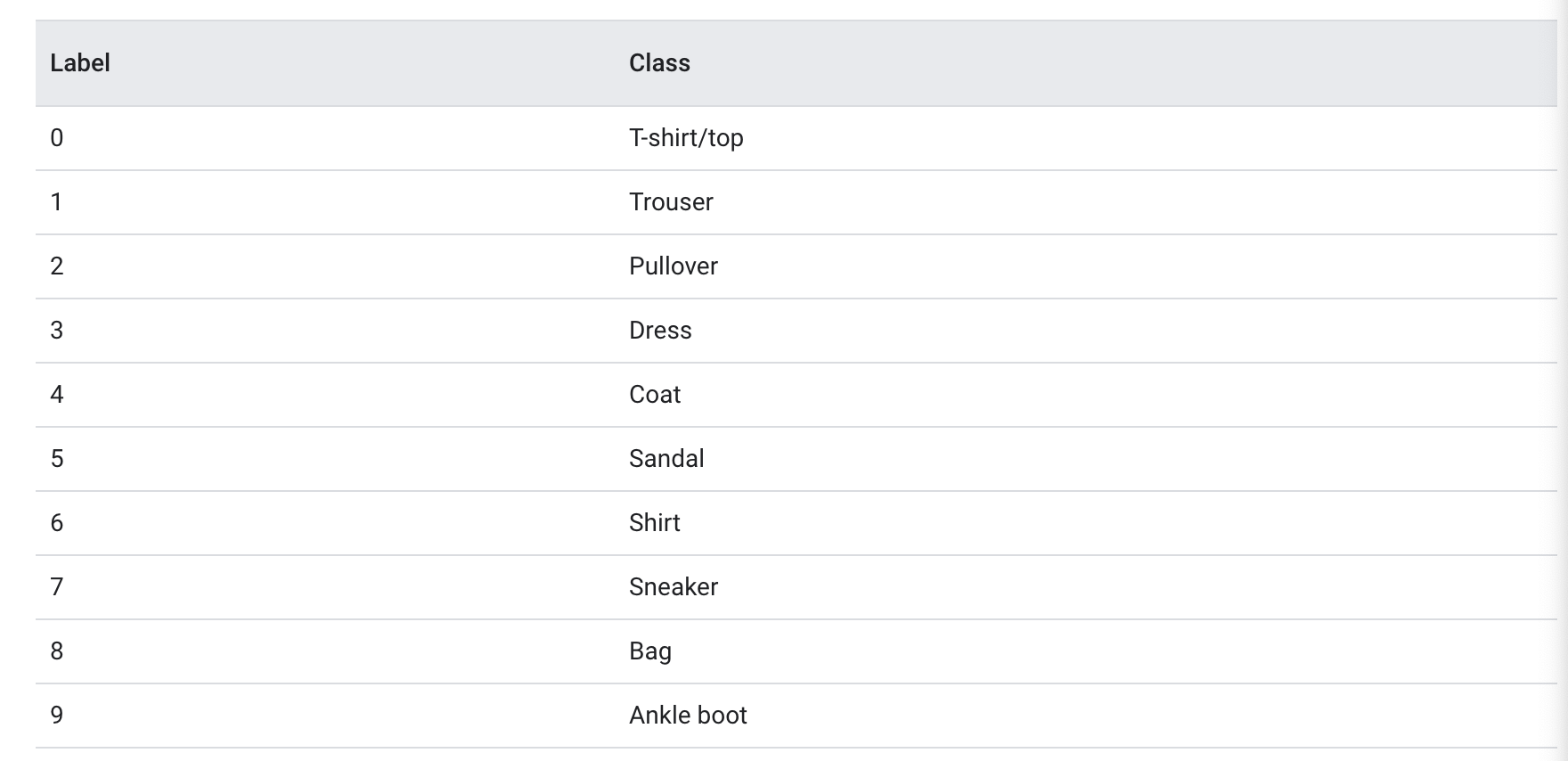
Since class names are not included in the set, we can store them in a list:

由于类名称不包含在集合中，因此我们可以将它们存储在列表中：

class_names = ['T-shirt/top', 'Trouser', 'Pullover', 'Dress', 'Coat', 'Sandal', 'Shirt', 'Sneaker', 'Bag', 'Ankle boot']

Before training the model, let’s explore the set. In our train_images we have 60,000 images and in our train_labels, we have 60,000 labels. Each label is an integer between 0 and 9, as given by this code:

在训练模型之前，让我们探索一下集合。 在train_images我们有60,000张图像，在train_labels ，我们有60,000张标签。 每个标签都是0到9之间的整数，如以下代码所示：

train_labels
# output: 

Likewise, there are 10,000 images in the test set. As expected, there are also 10,000 test labels. Each image is represented as 28 x 28 pixels. Let’s now preprocess our data. We can start by inspecting the first image:

同样，测试集中有10,000张图像。 正如预期的那样，还有10,000个测试标签。 每个图像表示为28 x 28像素。 现在让我们预处理数据。 我们可以从检查第一张图片开始：

plt.figure()
plt.imshow(train_images[0])
plt.colorbar()
plt.grid(False)
plt.show()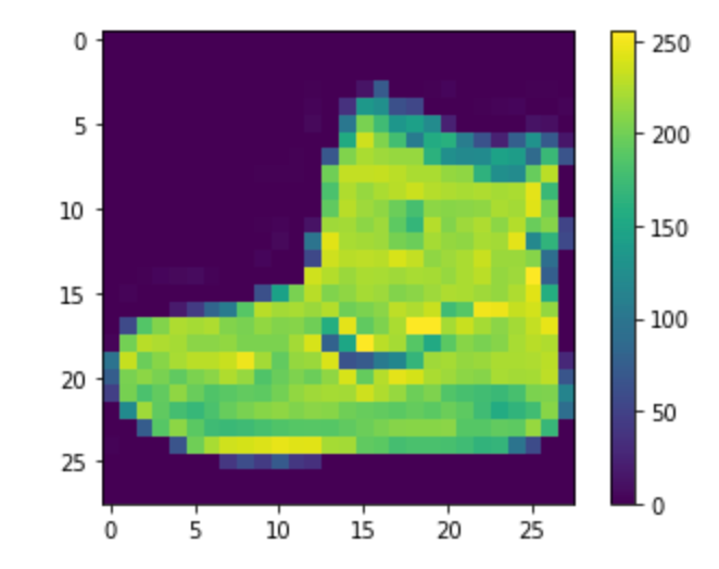

First Image

第一张图片

In this case, the pixel values fall between 0 and 255. Before feeding them into the neural network, we want them to be scaled between 0 and 1. To accomplish this, we can divide by 255 for both the training and testing set:

在这种情况下，像素值介于0到255之间。在将它们输入神经网络之前，我们希望它们在0到1之间缩放。要实现这一点，我们可以将训练集和测试集除以255：

train_images = train_images / 255.0
test_images = test_images / 255.0

Let’s verify if our data is now in the correct format. We can display the first 25 images from the training set and display the class name below each image:

让我们验证我们的数据现在是否采用正确的格式。 我们可以显示训练集中的前25个图像，并在每个图像下方显示班级名称：

plt.figure(figsize=(10,10))
for i in range(25):
    plt.subplot(5,5,i+1)
    plt.xticks([])
    plt.yticks([])
    plt.grid(False)
    plt.imshow(train_images[i], cmap=plt.cm.binary)
    plt.xlabel(class_names[train_labels[i]])
plt.show()

First 25 Images

前25张图片

Hooray, it worked! We are now ready to build our deep learning model. Since this is an image classification problem, we will need to use an artificial neural network. We will first need to configure the layers of our model, then compile the model. First, let’s configure our layers. Layers in a deep neural network extract representations from the data fed into them (). To set up our network, we will chain together a few layers. For this example, we will use the Sequential model:

太好了！ 现在，我们准备建立深度学习模型。 由于这是图像分类问题，因此我们需要使用人工神经网络。 我们首先需要配置模型的各层，然后编译模型。 首先，让我们配置我们的图层。 深度神经网络中的图层从输入到其中的数据中提取表示形式()。 为了建立我们的网络，我们将链接几层。 在此示例中，我们将使用顺序模型：

model = keras.Sequential([
    keras.layers.Flatten(input_shape=(28, 28)),
    keras.layers.Dense(128, activation='relu'),
    keras.layers.Dense(10)
])

The first layer in this network, tf.keras.layers.Flatten, transforms the format of images from 28 x 28 to a 1-D array of 784 pixels. Essentially, we are lining the pixels up. There is no learning in this layer, only reformatting. The next two layers in our network are tf.keras.layers.Dense layers. These are fully connected neural layers with 128 neurons. They return a score for whether the image belongs to one of the ten classes. Before we train our model, we need to add in the last step. While we compile the network we just built, we need to make sure that the performance is high! In other words, we want to minimize loss/training error. This code accomplishes the task:

该网络的第一层tf.keras.layers.Flatten将图像的格式从28 x 28转换为784像素的一维数组。 本质上，我们正在排列像素。 在这一层没有学习，只有重新格式化。 我们网络中的下两层是tf.keras.layers.Dense层。 这些是具有128个神经元的完全连接的神经层。 他们返回图像是否属于十个类别之一的分数。 在训练模型之前，我们需要在最后一步中添加。 在编译刚刚构建的网络时，我们需要确保性能很高！ 换句话说，我们要最小化损失/训练误差。 这段代码完成了任务：

model.compile(optimizer='adam',
           loss=tf.keras.losses.SparseCategoricalCrossentropy(from_logits=True,
              metrics=['accuracy'])

To do this, we employ a loss function to measure how accurate our model is during training. The goal will be to minimize this function. Our model is also compiled with an optimizer. This gives us a way to update our model based on loss. Finally, we compile with metrics. This is a way to monitor accuracy during the training and testing steps.

为此，我们使用损失函数来衡量模型在训练过程中的准确性。 目标是最小化此功能。 我们的模型也使用优化器进行编译。 这为我们提供了一种基于损失更新模型的方法。 最后，我们使用metrics进行编译。 这是在培训和测试步骤中监控准确性的方法。

We can now train our model:

我们现在可以训练我们的模型：

model.fit(train_images, train_labels, epochs=10)

Here, we feed in our training images and trining labels to the model as arrays. During training, we expect the model to associate images and labels. We can then ask our model to make predictions on the test set. Once we fit our model using the code above, you can expect an output like the following:

在这里，我们将训练图像和Trining标签作为数组输入模型。 在训练期间，我们希望模型能够关联图像和标签。 然后，我们可以要求我们的模型对测试集进行预测。 一旦我们使用上面的代码拟合了模型，您就可以期待如下输出：

Training of Model

模型训练

In this step, we see that our configured deep learning model trains for 10 epochs (10 training runs). In each epoch, it displays both the loss and accuracy. Since the model becomes better at recognizing different labels over time, the loss decreases and the performance increases across each epoch. At the final epoch (#10), our model reaches an accuracy of roughly 0.91 (91%). We can now take the final step to compare how the model performs on the test dataset:

在这一步中，我们看到我们配置的深度学习模型训练了10个时期(10次训练)。 在每个时期，它同时显示损失和准确性。 由于模型会随着时间的推移更好地识别不同的标签，因此在每个时期损失都将减少，性能也会提高。 在最后一个时期(＃10)，我们的模型达到约0.91(91％)的精度。 现在，我们可以采取最后一步来比较模型在测试数据集上的表现：

test_loss, test_acc = model.evaluate(test_images,  test_labels, verbose=2)
print('\nTest accuracy:', test_acc)

If we run this code, we find that our test accuracy was 0.884. You may be surprised that our training accuracy was higher than the test accuracy. The reason for this is simple: overfitting. Overfitting occurs when a machine learning model performs worse on unseen (testing) data due to highly specific training data. In other words, our model had memorized the noise and details of the training set to the point that it negatively impacts performance on new/testing data.

如果运行此代码，则会发现测试精度为0.884。 您可能会惊讶于我们的培训准确性高于测试准确性。 这样做的原因很简单： 过度拟合 。 当机器学习模型由于高度特定的训练数据而在看不见的(测试)数据上表现较差时，就会发生过度拟合。 换句话说，我们的模型已经记住了训练集的噪音和细节，以至于它会对新数据/测试数据的性能产生负面影响。

总结和最后的想法 (Summary and Final Thoughts)

Through this tutorial, you were able to learn and implement basic TensorFlow structures. We covered different data types, variables, placeholders, graphs, sessions, differences between 1.X and 2.X, eager execution, tensorboard, Keras, overfitting, etc! If you want to learn more and do more interesting projects/tutorials, be sure to check out tensorflow.org/tutorials. If you enjoyed reading, do be sure to give a clap :)

通过本教程，您可以学习和实现基本的TensorFlow结构。 我们介绍了不同的数据类型，变量，占位符，图形，会话，1.X和2.X之间的差异，热切的执行，张量板，Keras，过度拟合等！ 如果您想了解更多并且做更多有趣的项目/教程，请务必查看tensorflow.org/tutorials。 如果您喜欢阅读，请务必鼓掌:)

1. https://github.com/tensorflow/docs

   https://github.com/tensorflow/docs

2. https://www.tensorflow.org/tutorials/keras/classification (Keras Section is directly adapted from this tutorial)

   https://www.tensorflow.org/tutorials/keras/classification(Keras部分直接从本教程改编而来)

翻译自: https://medium.com/@siddrrsh/the-ultimate-beginners-guide-to-tensorflow-41d3b8e7d0c7

tensorflow入门