keras卷积网络图像分类_卷积神经网络进行图像处理—使用Keras

keras卷积网络图像分类

什么是图像分类？ (What is Image Classification?)

Image classification is the process of segmenting images into different categories based on their features. A feature could be the edges in an image, the pixel intensity, the change in pixel values, and many more. We will try and understand these components later on. For the time being let’s look into the images below (refer to Figure 1). The three images belong to the same individual however varies when compared across features like the color of the image, position of the face, the background color, color of the shirt, and many more. The biggest challenge when working with images is the uncertainty of these features. To the human eye, it looks all the same, however, when converted to data you may not find a specific pattern across these images easily.

图像分类是根据图像的特征将图像划分为不同类别的过程。 特征可能是图像的边缘，像素强度，像素值的变化等等。 稍后我们将尝试并理解这些组件。 现在，让我们看一下下面的图像(请参见图1)。 这三幅图像属于同一个人，但是在不同特征(例如图像的颜色，脸部位置，背景颜色，衬衫的颜色等)之间进行比较时，它们会有所不同。 使用图像时最大的挑战是这些功能的不确定性。 在人眼中，它看起来完全一样，但是，当转换为数据时，可能无法轻松地在这些图像上找到特定的图案。

Figure 1. Illustrates the portrait of the Author taken in 2014 and 2019 respectively.

图1.分别显示了2014年和2019年拍摄的作者肖像。

An image consists of the smallest indivisible segments called pixels and every pixel has a strength often known as the pixel intensity. Whenever we study a digital image, it usually comes with three color channels, i.e. the Red-Green-Blue channels, popularly known as the “RGB” values. Why RGB? Because it has been seen that a combination of these three can produce all possible color pallets. Whenever we work with a color image, the image is made up of multiple pixels with every pixel consisting of three different values for the RGB channels. Let’s code and understand what we are talking about.

图像由称为像素的最小不可分割的部分组成，每个像素的强度通常称为像素强度。 每当我们研究数字图像时，通常都会带有三个颜色通道，即红绿蓝通道，通常称为“ RGB”值。 为什么是RGB？ 因为已经看到这三种的组合可以生产所有可能的颜色托盘。 每当我们处理彩色图像时，图像都是由多个像素组成的，每个像素都由RGB通道的三个不同值组成。 让我们编写代码并了解我们在说什么。

import cv2
import seaborn as sns
import matplotlib.pyplot as plt
%matplotlib inline
sns.set(color_codes=True)# Read the image
image = cv2.imread('Portrait-Image.png') #--imread() helps in loading an image into jupyter including its pixel valuesplt.imshow(cv2.cvtColor(image, cv2.COLOR_BGR2RGB))
# as opencv loads in BGR format by default, we want to show it in RGB.
plt.show()image.shape

The output of image.shape is (450, 428, 3). The Shape of the image is 450 x 428 x 3 where 450 represents the height, 428 the width, and 3 represents the number of color channels. When we say 450 x 428 it means we have 192,600 pixels in the data and every pixel has an R-G-B value hence 3 color channels.

image.shape的输出为(450，428，3)。 图像的形状为450 x 428 x 3，其中450代表高度，428代表宽度，3代表颜色通道的数量。 当我们说450 x 428时，表示数据中有192,600像素，每个像素都有RGB值，因此有3个颜色通道。

image[0][0]

image [0][0] provides us with the R-G-B values of the first pixel which are 231, 233, and 243 respectively.

图像[0] [0]为我们提供了第一个像素的RGB值，分别为231、233和243。

# Convert image to grayscale. The second argument in the following step is cv2.COLOR_BGR2GRAY, which converts colour image to grayscale.
gray = cv2.cvtColor(image, cv2.COLOR_BGR2GRAY)
print(“Original Image:”)plt.imshow(cv2.cvtColor(gray, cv2.COLOR_BGR2RGB))
# as opencv loads in BGR format by default, we want to show it in RGB.
plt.show()gray.shape

The output of gray.shape is 450 x 428. What we see right now is an image consisting of 192,600 odd pixels but consists of one channel only.

gray.shape的输出为450 x428。我们现在看到的图像是由192,600个奇数像素组成，但仅包含一个通道。

When we try and covert the pixel values from the grayscale image into a tabular form this is what we observe.

当我们尝试将灰度图像的像素值转换为表格形式时，这就是我们观察到的。

import numpy as np
data = np.array(gray)
flattened = data.flatten()flattened.shape

Output: (192600,)

输出：(192600，)

We have the grayscale value for all 192,600 pixels in the form of an array.

我们以阵列形式获得所有192,600像素的灰度值。

flattened

Output: array([236, 238, 238, ..., 232, 231, 231], dtype=uint8). Note a grayscale value can lie between 0 to 255, 0 signifies black and 255 signifies white.

输出：array([236，238，238，...，232，231，231]，dtype = uint8)。 请注意，灰度值可以介于0到255之间，0表示黑色，255表示白色。

Now if we take multiple such images and try and label them as different individuals we can do it by analyzing the pixel values and looking for patterns in them. However, the challenge here is that since the background, the color scale, the clothing, etc. vary from image to image, it is hard to find patterns by analyzing the pixel values alone. Hence we might require a more advanced technique that can detect these edges or find the underlying pattern of different features in the face using which these images can be labeled or classified. This where a more advanced technique like CNN comes into the picture.

现在，如果我们拍摄多个此类图像并尝试将其标记为不同的个体，则可以通过分析像素值并在其中查找图案来实现。 然而，这里的挑战在于，由于背景，色阶，衣服等在图像之间变化，因此仅通过分析像素值很难找到图案。 因此，我们可能需要一种更高级的技术，该技术可以检测这些边缘或找到面部不同特征的基础图案，从而可以对这些图像进行标记或分类。 这是像CNN这样更先进的技术出现的地方。

什么是CNN？ (What is CNN?)

CNN or the convolutional neural network (CNN) is a class of deep learning neural networks. In short think of CNN as a machine learning algorithm that can take in an input image, assign importance (learnable weights and biases) to various aspects/objects in the image, and be able to differentiate one from the other.

CNN或卷积神经网络(CNN)是一类深度学习神经网络 。 简而言之，将CNN视为一种机器学习算法，可以获取输入图像，为图像中的各个方面/对象分配重要性(可学习的权重和偏差)，并能够区分彼此。

CNN works by extracting features from the images. Any CNN consists of the following:

CNN通过从图像中提取特征来工作。 任何CNN均包含以下内容：

1. The input layer which is a grayscale image
   输入层是灰度图像
2. The Output layer which is a binary or multi-class labels
   输出层是二进制或多类标签
3. Hidden layers consisting of convolution layers, ReLU (rectified linear unit) layers, the pooling layers, and a fully connected Neural Network
   隐藏层由卷积层，ReLU(整流线性单元)层，池化层和完全连接的神经网络组成

It is very important to understand that ANN or Artificial Neural Networks, made up of multiple neurons is not capable of extracting features from the image. This is where a combination of convolution and pooling layers comes into the picture. Similarly, the convolution and pooling layers can’t perform classification hence we need a fully connected Neural Network.

了解由多个神经元组成的ANN或人工神经网络无法从图像中提取特征非常重要。 这是卷积和池化层结合在一起的地方。 同样，卷积和池化层无法执行分类，因此我们需要一个完全连接的神经网络。

Before we jump into the concepts further let’s try and understand these individual segments separately.

在深入了解这些概念之前，让我们尝试分别了解这些单独的细分。

Figure 2. Illustrates the CNN process from input to Output Data. Image is taken from Slide 12, Introduction to Convolutional Neural Networks(Stanford University, 2018)

图2.说明了从输入到输出数据的CNN过程。 图片取自第12张幻灯片，卷积神经网络简介(斯坦福大学，2018年)

Let’s consider that we have access to multiple images of different vehicles, each labeled into a truck, car, van, bicycle, etc. Now the idea is to take these pre-label/classified images and develop a machine learning algorithm that is capable of accepting a new vehicle image and classify it into its correct category or label. Now before we start building a neural network we need to understand that most of the images are converted into a grayscale form before they are processed.

让我们考虑一下，我们可以访问不同车辆的多个图像，每个图像都标记为卡车，汽车，货车，自行车等。现在的想法是获取这些预先标记/分类的图像，并开发一种能够接受新的车辆图像并将其分类为正确的类别或标签。 现在，在开始构建神经网络之前，我们需要了解，大多数图像在处理之前都已转换为灰度形式。

为什么是灰度而不是RGB /彩色图像？ (Why grayscale and not RGB/Color Images?)

Figure 3. RGB color channels of an image. Image credits — Saha, S. (2018)

图3.图像的RGB颜色通道。 图片来源-Saha，S.(2018)

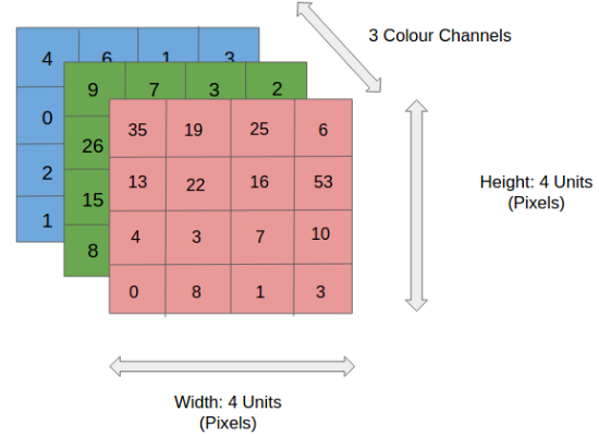
We discussed earlier that any color image has three channels, i.e. red, green, and blue as shown in Figure 3. There are several such color spaces like the grayscale, CMYK, HSV in which an image can exist.

前面我们讨论过，任何彩色图像都具有三个通道，即红色，绿色和蓝色，如图3所示。在其中可以存在图像的灰度级，CMYK，HSV等几种颜色空间。

The challenge with images having multiple color channels is that we have huge volumes of data to work with which makes the process computationally intensive. In other worlds think of it like a complicated process where the Neural Network or any machine learning algorithm has to work with three different data (R-G-B values in this case) to extract features of the images and classify them into their appropriate categories.

具有多个颜色通道的图像所面临的挑战是，我们需要处理大量数据，这使过程的计算量很大。 在其他世界中，这就像一个复杂的过程，其中神经网络或任何机器学习算法都必须使用三个不同的数据(在这种情况下为RGB值)来提取图像的特征并将其分类为适当的类别。

The role of CNN is to reduce the images into a form that is easier to process, without losing features critical towards a good prediction. This is important when we need to make the algorithm scalable to massive datasets.

CNN的作用是将图像缩小为易于处理的形式，而不会丢失对良好预测至关重要的功能。 当我们需要使算法可扩展到海量数据集时，这一点很重要。

什么是卷积？ (What are convolutions?)

演示地址

GIPHY GIPHY进行 GIF

We understand that the training data consists of grayscale images which will be an input to the convolution layer to extract features. The convolution layer consists of one or more Kernels with different weights that are used to extract features from the input image. Say in the example above we are working with a Kernel (K) of size 3 x 3 x 1 (x 1 because we have one color channel in the input image), having weights outlined below.

我们了解到，训练数据由灰度图像组成，这将是卷积层提取特征的输入。 卷积层由一个或多个具有不同权重的内核组成，用于从输入图像中提取特征。 在上面的示例中说，我们正在使用尺寸为3 x 3 x 1(x 1，因为我们在输入图像中有一个颜色通道)的内核(K)，其权重如下所示。

Kernel/Filter, K = 
1  0  1
0  1  0
1  0  1

When we slide the Kernel over the input image (say the values in the input image are grayscale intensities) based on the weights of the Kernel we end up calculating features for different pixels based on their surrounding/neighboring pixel values. E.g. when the Kernel is applied on the image for the first time as illustrated in Figure 5 below we get a feature value equal to 4 in the convolved feature matrix as shown below.

当我们基于内核的权重在输入图像上滑动内核(例如，输入图像中的值是灰度强度)时，最终我们会基于周围/相邻像素值为不同像素计算特征。 例如，当将内核第一次应用于图像时，如下图5所示，在卷积特征矩阵中我们得到的特征值等于4，如下所示。

Figure 5. Illustrated the value of the convolved feature when the Kernel is applied to the input image. The image is a snapshot of the GIF used in Figure 4 above.

图5.说明了将内核应用于输入图像时卷积特征的值。 该图像是上面图4中使用的GIF的快照。

If we observe Figure 4 carefully we will see that the kernel shifts 9 times across image. This process is called Stride. When we use a stride value of 1 (Non-Strided) operation we need 9 iterations to cover the entire image. The CNN learns the weights of these Kernels on its own. The result of this operation is a feature map that basically detects features from the images rather than looking into every single pixel value.

如果仔细观察图4，我们将看到内核在整个图像上移动了9次。 此过程称为跨步。 当我们使用跨步值1( Non-Strided )操作时，我们需要9次迭代才能覆盖整个图像。 CNN会自行学习这些内核的权重。 此操作的结果是一个特征图，该特征图基本上从图像中检测特征，而不是查看每个像素值。

I

一世

让我们更深入地了解我们在说什么。 (Let’s take a deeper look into what we are talking about.)

Extracting features from an image is similar to detecting edges in the image. We can use the openCV package to perform the same. We will declare a few matrices, apply them on a grayscale image, and try and look for edges. You can find more about the function here.

从图像中提取特征类似于检测图像中的边缘。 我们可以使用openCV包执行相同的操作。 我们将声明一些矩阵，将它们应用于灰度图像，然后尝试寻找边缘。 您可以在此处找到有关该功能的更多信息。

# 3x3 array for edge detection
mat_y = np.array([[ -1, -2, -1], 
                   [ 0, 0, 0], 
                   [ 1, 2, 1]])
mat_x = np.array([[ -1, 0, 1], 
                   [ 0, 0, 0], 
                   [ 1, 2, 1]])
  
filtered_image = cv2.filter2D(gray, -1, mat_y)
plt.imshow(filtered_image, cmap='gray')filtered_image = cv2.filter2D(gray, -1, mat_x)
plt.imshow(filtered_image, cmap='gray')

Figure 6. Illustrates images with edges when a filter2D transformation is applied to the data. Note that the two images are significantly different. When we talk about convolution layers and Kernels we basically want to identify the edges in an image. When working with CNN the matrix_x and matrix_y values are determined automatically by the network. Image taken from the Jupyter Notebook developed by the Author.

图6.说明了将filter2D转换应用于数据时带有边缘的图像。 请注意，这两个图像明显不同。 当我们谈论卷积层和核时，我们基本上要确定图像中的边缘。 使用CNN时，matrix_x和matrix_y值由网络自动确定。 图片取自作者开发的Jupyter笔记本。

import torch
import torch.nn as nn
import torch.nn.functional as fn

If you are working with windows install the following — # conda install pytorch torchvision cudatoolkit=10.2 -c pytorch for using pytorch.

如果使用Windows，请安装以下软件—＃conda install pytorch torchvision cudatoolkit = 10.2 -c pytorch以使用pytorch。

import numpy as np
filter_vals = np.array([[-1, -1, 1, 2], [-1, -1, 1, 0], [-1, -1, 1, 1], [-1, -1, 1, 1]])
print(‘Filter shape: ‘, filter_vals.shape)# Neural network with one convolutional layer and four filters
class Net(nn.Module):
 
 def __init__(self, weight): #Declaring a constructor to initialize the class variables
 super(Net, self).__init__()
 # Initializes the weights of the convolutional layer to be the weights of the 4 defined filters
 k_height, k_width = weight.shape[2:]
 # Assumes there are 4 grayscale filters; We declare the CNN layer here. Size of the kernel equals size of the filter
 # Usually the Kernels are smaller in size
 self.conv = nn.Conv2d(1, 4, kernel_size=(k_height, k_width), bias=False)
 self.conv.weight = torch.nn.Parameter(weight)
 
 def forward(self, x):
 # Calculates the output of a convolutional layer pre- and post-activation
 conv_x = self.conv(x)
 activated_x = fn.relu(conv_x)# Returns both layers
 return conv_x, activated_x# Instantiate the model and set the weights
weight = torch.from_numpy(filters).unsqueeze(1).type(torch.FloatTensor)
model = Net(weight)# Print out the layer in the network
print(model)

We create the visualization layer, call the class object, and display the output of the Convolution of four kernels on the image (Bonner, 2019).

我们创建可视化层，调用class对象，并在图像上显示四个内核的卷积的输出(Bonner，2019)。

def visualization_layer(layer, n_filters= 4):
    
    fig = plt.figure(figsize=(20, 20))
    
    for i in range(n_filters):
        ax = fig.add_subplot(1, n_filters, i+1, xticks=[], yticks=[])
        # Grab layer outputs
        ax.imshow(np.squeeze(layer[0,i].data.numpy()), cmap='gray')
        ax.set_title('Output %s' % str(i+1))

The convolution operation.

卷积运算。

#-----------------Display the Original Image------------------- 
plt.imshow(gray, cmap='gray')#-----------------Visualize all of the filters------------------
fig = plt.figure(figsize=(12, 6))
fig.subplots_adjust(left=0, right=1.5, bottom=0.8, top=1, hspace=0.05, wspace=0.05)for i in range(4):
    ax = fig.add_subplot(1, 4, i+1, xticks=[], yticks=[])
    ax.imshow(filters[i], cmap='gray')
    ax.set_title('Filter %s' % str(i+1))
    
# Convert the image into an input tensor
gray_img_tensor = torch.from_numpy(gray).unsqueeze(0).unsqueeze(1)
# print(type(gray_img_tensor))# print(gray_img_tensor)# Get the convolutional layer (pre and post activation)
conv_layer, activated_layer = model.forward(gray_img_tensor.float())# Visualize the output of a convolutional layer
visualization_layer(conv_layer)

Output:

输出：

Figure 7. Illustrates the output of different filters on the original gray scale image. Snap shot is generated using Jupyter Notebook and the above codes.

图7.说明了原始灰度图像上不同滤镜的输出。 快照是使用Jupyter Notebook和上面的代码生成的。

Note: Depending on the weights associated with a filter, the features are detected from the image. Notice when an image is passed through a convolution layer, it and tries and identify the features by analyzing the change in neighboring pixel intensities. E.g. the top right of the image has similar pixel intensity throughout, hence no edges are detected. It is only when the pixels change intensity the edges are visible.

注意：根据与滤镜相关的权重，将从图像中检测到特征。 请注意，当图像通过卷积层时，它会通过分析相邻像素强度的变化来尝试识别特征。 例如，图像的右上方始终具有相似的像素强度，因此未检测到边缘。 只有当像素改变强度时，边缘才可见。

为什么选择ReLU？ (Why ReLU?)

ReLU or rectified linear unit is a process of applying an activation function to increase the non-linearity of the network without affecting the receptive fields of convolution layers. ReLU allows faster training of the data, whereas Leaky ReLU can be used to handle the problem of vanishing gradient. Some of the other activation functions include Leaky ReLU, Randomized Leaky ReLU, Parameterized ReLU Exponential Linear Units (ELU), Scaled Exponential Linear Units Tanh, hardtanh, softtanh, softsign, softmax, and softplus.

ReLU或整流线性单位是应用激活函数以增加网络的非线性而不影响卷积层的接收场的过程。 ReLU可以更快地训练数据，而Leaky ReLU可用于解决梯度消失的问题。 其他一些激活功能包括泄漏ReLU，随机泄漏ReLU，参数化ReLU指数线性单位(ELU)，比例指数线性单位Tanh，hardtanh，softtanh，softsign，softmax和softplus。

演示地址

Figure 8. Illustrates the impact of ReLU and how it removes non-linearity by converting negatives to zeros. Image credit — GIF via Gfycat.

图8.说明了ReLU的影响以及它如何通过将负数转换为零来消除非线性。 图片信用-通过Gfycat的GIF。

visualization_layer(activated_layer)

Figure 9. Illustrates the output of the Convolution layer followed by a ReLU activation. Image taken from the Jupyter Notebook developed by the Author.

图9.展示了卷积层的输出以及随后的ReLU激活。 图片取自作者开发的Jupyter笔记本。

Figure 10. Illustrates how kernels work with an image that has R-G-B channels. Image credits — Saha, S. (2018)

图10.说明内核如何处理具有RGB通道的图像。 图片来源-Saha，S.(2018)

Figure 11. Application of a 3 x 3 Kernel on a 5 x 5 Image. Image credits (Visin, 2016)

图11.在5 x 5图像上应用3 x 3内核。 图片学分(Visin，2016)

The general objective of the convolution operation is to extract high-level features from the image. We can always add more than one convolution layer when building the neural network, where the first Convolution Layer is responsible for capturing gradients whereas the second layer captures the edges. The addition of layers depends on the complexity of the image hence there are no magic numbers on how many layers to add. Note application of a 3 x 3 filter results in the original image results in a 3 x 3 convolved feature, hence to maintain the original dimension often the image is padded with values on both ends.

卷积运算的总体目标是从图像中提取高级特征。 在构建神经网络时，我们总是可以添加多个卷积层，其中第一卷积层负责捕获梯度，而第二层卷积边缘。 层的增加取决于图像的复杂性，因此在增加多少层上没有神奇的数字。 请注意，使用3 x 3滤镜会导致原始图像产生3 x 3卷积特征，因此为了保持原始尺寸，通常会在图像的两端都填充值。

池层的作用 (Role of the Pooling Layer)

The pooling layer applies a non-linear down-sampling on the convolved feature often referred to as the activation maps. This is mainly to reduce the computational complexity required to process the huge volume of data linked to an image. Pooling is not compulsory and is often avoided. Usually, there are two types of pooling, Max Pooling, that returns the maximum value from the portion of the image covered by the Pooling Kernel and the Average Pooling that averages the values covered by a Pooling Kernel. Figure 12 below provides a working example of how different pooling techniques work.

池化层对卷积特征进行非线性下采样，该卷积特征通常称为激活图 。 这主要是为了减少处理链接到图像的大量数据所需的计算复杂性。 池化不是强制性的，通常可以避免。 通常，池化有两种类型：“ 最大池化”( Max Pooling)和“ 平均池化 ”( Average Pooling) ，该值从池化内核覆盖的图像部分返回最大值，而“ 平均池化”将池化内核覆盖的值取平均值。 下面的图12提供了一个不同的池技术如何工作的工作示例。

Figure 12. Illustrates how Maximum & Average Pooling is carried out on the activation maps. Image is taken from Slide 18, Introduction to Convolutional Neural Networks(Stanford University, 2018)

图12.说明了如何在激活图上执行最大池和平均池。 图片摘自第18页，卷积神经网络简介(斯坦福大学，2018年)

图像展平 (Image Flattening)

Once the pooling is done the output needs to be converted to a tabular structure that can be used by an artificial neural network to perform the classification. Note the number of the dense layer as well as the number of neurons can vary depending on the problem statement. Also often a drop out layer is added to prevent overfitting of the algorithm. Dropouts ignore few of the activation maps while training the data however use all activation maps during the testing phase. It prevents overfitting by reducing the correlation between neurons.

合并完成后，需要将输出转换为表格结构，人工神经网络可以使用该表格结构执行分类。 请注意，致密层的数量以及神经元的数量可能会根据问题陈述而有所不同。 同样经常会添加一个辍学层，以防止算法过度拟合。 在训练数据时，辍学忽略很少的激活图，但是在测试阶段将使用所有激活图。 它通过减少神经元之间的相关性来防止过度拟合。

here. 此处找到。

使用CIFAR-10数据集 (Working with the CIFAR-10 dataset)

An end to end example of working with CNN using Keras is provided in the link below.

下面的链接中提供了使用Keras使用CNN的端到端示例。

About the Author: Advanced analytics professional and management consultant helping companies find solutions for diverse problems through a mix of business, technology, and math on organizational data. A Data Science enthusiast, here to share, learn and contribute; You can connect with me on Linked and Twitter;

作者简介：高级分析专家和管理顾问，通过组织数据的业务，技术和数学相结合，帮助公司找到各种问题的解决方案。 数据科学爱好者，在这里分享，学习和贡献； 您可以在 Linked 和 Twitter上 与我 联系 ；

翻译自: https://towardsdatascience.com/convolution-neural-network-for-image-processing-using-keras-dc3429056306

keras卷积网络图像分类