激活函数,优化技术和损失函数

激活功能: (Activation Functions:)

A significant piece of a neural system Activation function is numerical conditions that decide the yield of a neural system. The capacity is joined to every neuron in the system and decides if it ought to be initiated (“fired”) or not, founded on whether every neuron’s info is applicable for the model’s expectation. Initiation works likewise help standardize the yield of every neuron to a range somewhere in the range of 1 and 0 or between — 1 and 1.

神经系统的重要部分激活函数是决定神经系统产量的数值条件。 该能力与系统中的每个神经元相连,并根据每个神经元的信息是否适用于模型的期望来决定是否应该启动(“发射”)该能力。 初始化工作同样有助于将每个神经元的产量标准化到介于1到0或介于1到1的范围内。

Progressively, neural systems use linear and non-linear activation functions, which can enable the system to learn complex information, figure and adapt practically any capacity speaking to an inquiry, and give precise forecasts.

神经系统逐渐地使用线性和非线性激活函数,这可以使系统学习复杂的信息,计算和适应几乎所有与查询相关的能力,并给出精确的预测。

线性激活功能: (Linear Activation Functions:)

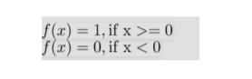
Step-Up: Activation functions are dynamic units of neural systems. They figure the net yield of a neural node. In this, Heaviside step work is one of the most widely recognized initiation work in neural systems. The capacity produces paired yield. That is the motivation behind why it is additionally called paired advanced capacity.

升压:激活函数是神经系统的动态单位。 他们计算出神经节点的净产量。 在这种情况下,Heaviside步骤工作是神经系统中最广泛认可的启动工作之一。 容量产生成对的产量。 这就是为什么将其另外称为成对高级容量的原因。

The capacity produces 1 (or valid) when info passes edge limit though it produces 0 (or bogus) when information doesn’t pass edge. That is the reason, they are extremely valuable for paired order studies. Every rationale capacity can be actualized by neural systems. In this way, step work is usually utilized in crude neural systems without concealed layer or generally referred to name as single-layer perceptions.

当信息通过边缘限制时,容量将生成1(或有效),但当信息未通过边缘时,容量将生成0(或虚假)。 这就是原因,它们对于配对订单研究非常有价值。 神经系统可以实现每个基本能力。 这样,通常在没有隐藏层的粗神经系统中使用步进工作,或通常将其称为单层感知。

  • The simplest kind of activation function

    最简单的激活功能
  • consider a threshold value and if the value of net input say x is greater than the threshold then the neuron is activated

    考虑一个阈值,如果净输入值x大于阈值,则激活神经元
Image for post
Step-Up Function
升压功能

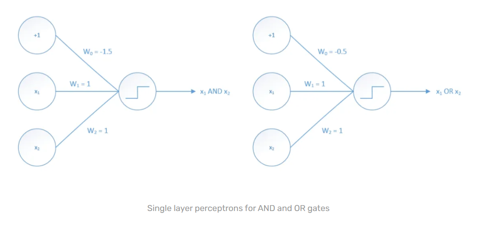
This kind of system can group straightly distinguishable issues, for example, AND-GATE and OR-GATE. As it were, all classes (0 and 1) can be isolated by a solitary straight line as outlined underneathAssume that we got edge an incentive as 0. After that point, the accompanying single layer neural system models will fulfill these rationale capacities.

这种系统可以将可直接区分的问题分组,例如AND-GATE和OR-GATE。 照原样,所有类别(0和1)都可以通过一条孤立的直线来隔离,如下所述。假定我们将边激励设为0。此后,随附的单层神经系统模型将满足这些基本要求。

Image for post
AND-GATE and OR-GATE
AND-GATE和OR-GATE

However, a linear activation function has two major problems:

但是,线性激活函数有两个主要问题:

  1. Unrealistic to utilize backpropagation (slope plunge) to prepare the model — the subordinate of the capacity is consistent, and has no connection to the info, X. So it’s impractical to return and comprehend which loads in the information neurons can give a superior expectation.

    利用反向传播 (斜率下降)来准备模型是不现实的-容量的下属是一致的,并且与信息X没有关系。因此,返回和理解信息神经元中的哪些负载可以给出更高的期望是不切实际的。

  2. All layers of the neural network collapse into one with linear activation functions, no matter how many layers in the neural network, the last layer will be a linear function of the first layer (because a linear combination of linear functions is still a linear function). So a linear activation function turns the neural network into just one layer.

    神经网络的所有层都折叠成具有线性激活函数的层,无论神经网络中有多少层,最后一层将是第一层的线性函数(因为线性函数的线性组合仍然是线性函数) 。 因此,线性激活函数将神经网络变成仅一层。

非线性激活功能: (Non-Linear Activation Functions:)

Present-day neural system models use non-straight activation capacities. They permit the model to make complex mappings between the system’s sources of info and yields, which are basic for learning and demonstrating complex information, for example, pictures, video, sound, and informational indexes which are non-straight or have high dimensionality.

当今的神经系统模型使用非直线激活能力。 它们允许模型在系统的信息源和收益之间进行复杂的映射,这对于学习和演示复杂的信息(例如图片,视频,声音和非直线或具有高维的信息索引)是基本的。

Practically any procedure conceivable can be spoken to as a useful calculation in a neural system, given that the initiation work is non-straight. Non-straight capacities address the issues of a direct enactment work: They permit backpropagation since they have a subordinate capacity which is identified with the information sources. They permit the “stacking” of various layers of neurons to make a profound neural system.

考虑到启动工作是非直线的,实际上任何可以想到的过程都可以说成是神经系统中的有用计算。 非直接能力解决了直接制定工作的问题:它们允许反向传播,因为它们具有从信息源中识别出的从属能力。 它们允许“堆叠”神经元的各个层以构成一个深奥的神经系统。

Different shrouded layers of neurons are expected to learn complex informational indexes with significant levels of exactness. Thus, types of non-linear activation functions are:

期望神经元的不同覆盖层学习具有显着水平的准确性的复杂信息索引。 因此,非线性激活函数的类型为:

  1. SIGMOID:

    SIGMOID:

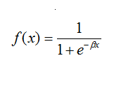
The fundamental motivation behind why we utilize the sigmoid capacity is that it exists between (0 to 1). In this manner, it is particularly utilized for models where we need to foresee the likelihood as a yield. Since the likelihood of anything exists just between the scope of 0 and 1, sigmoid is the correct decision.

我们为什么使用S形容量的根本动机是它存在于(0到1)之间。 以这种方式,它特别适用于需要预测可能性为收益的模型。 由于任何事情的可能性都介于0和1的范围之间,因此S型是正确的决定。

Image for post
Sigmoid-Function
乙状结肠功能

Advantages:

优点:

  • Smooth slope, forestalling “bounces” in yield esteems.

    平滑的坡度,阻止屈服感的“反弹”。
  • Output values bound somewhere in the range of 0 and 1, normalizing the yield of every neuron.

    输出值的范围在0到1之间,使每个神经元的产量正常化。
  • Clear forecasts — For X over 2 or beneath — 2, will in general bring the Y esteem (the expectation) to the edge of the bend, exceptionally near 1 or 0. This empowers clear expectations.

    明确的预测-对于大于2或小于2的X,通常会将Y估计(期望)带到弯道的边缘,特别是接近1或0。这将带来明确的期望。

Disadvantages:

缺点:

  • Vanishing Gradient — for exceptionally high or low estimations of X, there is practically no change to the forecast, causing a disappearing slope issue. This can bring about the system declining to learn further or being too delayed to even think about reaching an exact forecast.

    消失梯度-对于X的极高或极低的估计,预测几乎没有变化,从而导致斜率问题逐渐消失。 这可能会导致系统拒绝进一步学习或太迟甚至无法考虑达到准确的预测。
  • Outputs not zero focused and computationally costly.

    输出不是集中于零的,并且计算成本很高。
Image for post
Sigmoid-Curve
乙状弯曲

2. TANH:

2. TANH:

The tanh work is characterized as follows: It is nonlinear, so we can stack layers. It is bound to the range (- 1, 1) The angle is more grounded for tanh than sigmoid ( subordinates are more extreme) Like sigmoid, tanh additionally has an evaporating inclination issue.

tanh工作的特征如下:它是非线性的,因此我们可以堆叠图层。 它限制在范围(-1,1)中,与sigmoid相比,tanh的角度更接地(下属更极端)像sigmoid一样,tanh还具有蒸发倾斜的问题。

Advantages

优点

  • Zero centered making it easier to model inputs that have strongly negative, neutral, and strongly positive values.

    零位居中使得更容易对具有强负,中性和强正值的输入进行建模。

  • Otherwise like the Sigmoid function.

    否则就像Sigmoid函数。

Disadvantages

缺点

  • Like the Sigmoid function

    像Sigmoid函数
Image for post
Tanh-Function
正切函数

3. Rectified Linear Unit( RELU):

3. 整流线性单位( RELU):

In arithmetic a capacity is viewed as straight at whatever point a function f: A→B if for each x and y in the area A has the accompanying property: f(x)+f(y)=f(x+y). By definition the ReLU is max(0,x). Accordingly, if we split the area from (−∞,0] or [0,∞) at that point the capacity is straight. Be that as it may, it’s anything but difficult to see that f(−1)+f(1)≠f(0). Subsequently, by definition, ReLU isn’t straight.

在算术中,将容量视为函数f的任意点处的直线:如果A区域中的每个x和y具有伴随属性:f(x)+ f(y)= f(x + y),则A→B。 根据定义,ReLU为max(0,x)。 因此,如果我们在那个点从(-∞,0]或[0,∞)划分面积,则容量是直的。 尽管如此,要看到f(-1)+ f(1)≠f(0)还是很困难的。 随后,根据定义,ReLU不是直截了当的。

Image for post
ReLU-Function
ReLU功能

By and by, ReLU is so near straight this frequently befuddles individuals and miracle how might it be utilized as an all-inclusive approximator. I would say, the most ideal approach to consider them resembles Riemann wholes. You can inexact any consistent capacities with bunches of little square shapes. ReLU initiations can create bunches of little square shapes. Truth be told, practically speaking, ReLU can make rather confusing shapes and estimated many entangled areas.

渐渐地,ReLU变得如此直率,这经常使个人困惑,并奇迹般地将其用作一个包罗万象的近似器。 我想说,考虑它们的最理想方法类似于黎曼整体。 您可以用一堆小正方形来折衷任何一致的容量。 ReLU引发可以创建一堆小正方形。 说实话,实际上,ReLU可以使形状变得相当混乱,并可以估计许多纠缠区域。

I likewise want to explain another point. As brought up by a past answer, neurons don’t bite the dust in Sigmoid, but instead, evaporate. The purpose behind this is because at greatest the subordinate of the sigmoid capacity is .25. Henceforth, after such a large number of layers you wind up duplicating these angles and the result of exceptionally little numbers under 1 will in general go to zero rapidly.

我同样想解释另一点。 根据过去的回答,神经元不会咬住乙状结肠,而是会蒸发。 其背后的目的是因为乙状结肠容量的下位最大为.25。 从此以后,在经过如此多的层之后,您最终会重复这些角度,并且极少的数字小于1的结果通常会Swift变为零。

Subsequently, in case you’re constructing a profound learning system with a ton of layers, your sigmoid capacities will stale rather rapidly and turn out to be pretty much futile. The key remove is the evaporating originates from increasing the inclinations, not simply the slopes.

随后,如果您要构建一个具有大量层次的深刻的学习系统,则您的S形能力将很快失效,并且变得徒劳无益。 关键的去除是蒸发来自于倾斜度的增加,而不仅仅是倾斜。

Image for post
ReLU-Curve
ReLU曲线

Advantages

优点

  • Computationally proficient — permits the system to meet rapidly

    计算熟练-允许系统快速满足
  • Non-direct — even though it would seem that a straight capacity, ReLU has a subsidiary capacity and takes into account backpropagation

    非直接的-尽管ReLU似乎具有直接能力,但具有辅助能力并考虑了反向传播

Disadvantages

缺点

  • The Dying ReLU issue — when data sources approach zero or are negative, the angle of the capacity gets zero, the system can’t perform backpropagation and can’t learn.

    Dying ReLU问题–当数据源接近零或为负数时,容量角度为零,系统无法执行反向传播,也无法学习。

4. LEAKY-RELU

4. 渗漏

Image for post
Leaky-ReLU-Function
泄漏的ReLU功能

LEAKY ReLUs is one endeavor to fix the “perishing ReLU” issue. Rather than the capacity being zero when x < 0, a LEAKY ReLU will rather have a little negative slant (of 0.01, or thereabouts). That is, the capacity registers f(x)=1(x<0)(αx)+1(x>=0)(x) where α is a little consistent

漏水 ReLUs是解决“ peringing ReLU”问题的一项工作。 当x <0时,LEAKY ReLU的容量将为零,而不是零(0.01左右)。 也就是说,容量寄存器f(x)= 1(x <0)(αx)+1(x> = 0)(x),其中α有点一致

Image for post
Leaky-ReLU-Curve
泄漏的ReLU曲线

Advantages

优点

  • Prevents biting the dust ReLU issue — this variety of ReLU has a little positive slant in the negative region, so it empowers backpropagation, in any event, for negative information esteems

    防止咬住灰尘ReLU问题-这种ReLU在负区域有一些正向倾斜,因此无论如何,它都可以进行反向传播以获取负信息。
  • Otherwise like ReLU

    否则像ReLU

Disadvantages

缺点

  • Results not steady — LEAKY ReLU doesn’t give reliable forecasts to negative info esteems.

    结果不稳定-LEAKY ReLU无法对负面信息推崇可靠的预测。

优化功能 (Optimization Functions)

Gradient Descent Update Rule: Gradient descent is a streamlining calculation used to limit some capacity by iteratively moving toward the steepest drop as characterized by the negative of the slope. In AI, we use slope plunge to refresh the boundaries of our model. Boundaries allude to coefficients in Linear Regression and loads in neural systems.

梯度下降更新规则 :梯度下降是一种精简计算,用于通过迭代地向最陡峭的下降(以斜率的负数为特征)移动来限制某些容量。 在AI中,我们使用斜率下降来刷新模型的边界。 边界暗示线性回归中的系数和神经系统中的载荷。

Image for post
Walking-Down-Hill
步行下山

Beginning at the head of the mountain, we venture out toward the path determined by the negative inclination. Next, we recalculate the negative inclination (going in the directions of our new point) and make another stride toward the path it determines. We proceed with this procedure iteratively until we get to the base of our diagram, or to a point where we can no longer move downhill–a neighborhood least.

从山顶开始,我们朝着由负倾角确定的路径冒险。 接下来,我们重新计算负倾角(朝新点的方向),并朝着它确定的路径大步前进。 我们反复进行此过程,直到到达图的基础,或者到达无法再下坡的地步-最少。

Image for post
Gradient-Update-Rule_Function
渐变更新规则_功能

Learning rate: The size of these steps is known as the learning rate. With a high learning rate, we can make more progress each progression, however, we chance to overshoot the absolute bottom since the slant of the slope is continually evolving. With an exceptionally low learning rate, we can certainly move toward the negative slope since we are recalculating it so oftentimes. A low learning rate is more exact, however figuring the inclination is tedious, so it will take us a long effort to get to the base.

学习率:这些步骤的大小称为学习率。 有了较高的学习率,我们就可以在每个进度上取得更多的进步,但是,由于斜坡的倾斜度不断变化,因此我们有机会超过绝对的底部。 由于学习率极低,我们当然可以向负斜率移动,因为我们经常重新计算它。 较低的学习率更为准确,但是弄清这种倾向是乏味的,因此要想打基础,将需要我们花费很长时间。

Cost function: A Loss Functions lets us know “how great” our model is at making expectations for a given arrangement of boundaries. The cost of work has its bend and its slopes. The slant of this bend discloses to us how to refresh our boundaries to make the model more exact.

成本函数:损失函数使我们知道模型对给定的边界排列期望有多“出色”。 工作成本有其弯曲和倾斜。 此弯曲的倾斜向我们揭示了如何刷新边界以使模型更精确。

Step-by-step: Presently we should run gradient descent utilizing our new cost work. There are two boundaries in our cost work we can control: m (weight) and b (bias). Since we have to consider the effect everyone has on the last forecast, we have to utilize fractional subsidiaries. We compute the halfway subsidiaries of the cost work for every boundary and store the outcomes at an angle.

循序渐进:目前,我们应该利用新的成本工作进行梯度下降。 我们可以控制的成本工作有两个边界:m(权重)和b(偏差)。 由于我们必须考虑每个人对最新预测的影响,因此我们必须使用小数子公司。 我们为每个边界计算成本工作的中途子公司,并以一定角度存储结果。

Math

数学

Given the cost function:

给定成本函数:

Image for post
Cost-Function
成本函数

To solve for the gradient, we iterate through our data points using our new m and b values and compute the partial derivatives. This new gradient tells us the slope of our cost function at our current position (current parameter values) and the direction we should move to update our parameters. The size of our update is controlled by the learning rate.

为了解决梯度,我们使用新的m和b值遍历数据点并计算偏导数。 这个新的梯度告诉我们成本函数在当前位置(当前参数值)的斜率以及更新参数的方向。 我们更新的大小由学习率控制。

优化技术的类型: (Types Of Optimization Techniques:)

  1. Momentum Based GD:

    基于动量的GD:

  • Momentum based Gradient Descent Update Rule: One of the main issues​ with Gradient Descent is that it takes a lot of time to navigate regions with gentle slopes because the gradient is very small in these regions

    基于动量的梯度下降更新规则:梯度下降的主要问题之一是导航时需要花费很多时间,因为这些区域的梯度非常小
  • An intuitive solution​ would be that if the algorithm is repeatedly being asked to go in the same direction, then it should probably gain some confidence and start taking bigger steps in that direction

    直观的解决方案是,如果反复要求算法朝同一方向前进,那么它可能应该会获得一定的信心并开始朝该方向采取更大的措施
  • Now, we have to convert this intuition into a set of mathematical equations Gradient Descent Update Rule,

    现在,我们必须将这种直觉转换为一组数学方程式梯度下降更新规则,

ωt+1 = ωt — η∇ωt

ωt+ 1 =ωt—η∇ωt

→ υt = γ * υt−1 + η∇ωt

→υt=γ* υt−1 +η∇ωt

→ ωt+1 = ωt − υt

→ωt+ 1 =ωt−υt

→ ωt+1 = ωt − γ * υt−1 − η∇ωt

→ωt+ 1 =ωt−γ* υt−1 −η∇ωt

→ If γ * υt−1 = 0 then it is the same as the regular Gradient Descent update rule

→如果γ* υt−1 = 0,则它与常规梯度下降更新规则相同

→To put it briefly υt−1 is the history of the movement in a direction and γ ranges from 0–1

→简单地说,υt-1是一个方向的运动历史,并且γ的范围是0-1

A few points to note:

需要注意的几点:

a. Momentum based gradient descent oscillates in and out of the minima valley (u-turns)

一个。 基于动量的梯度下降在最小谷内摆动(u形转弯)

b. Despite these u-turns, it still converges faster than vanilla gradient descent

b。 尽管有这些掉头,但收敛速度仍比香草梯度下降快

Now, we will look at reducing the oscillations in Momentum based GD

现在,我们将着眼于减少基于动量的GD的振荡

2. Nesterov Accelerated Gradient Descent(NAG):

2. Nesterov加速梯度下降(NAG):

In Momentum based Gradient Descent, we can see that the movement occurs in two steps: The first is with the history-term γ * υt−1 and The second is with the weight term η∇ωt consider first moving with the history term, then calculate the second step from where we were located after the first step ( ωtemp ).

在基于动量的梯度下降中,我们可以看到运动发生在两个步骤中:第一步是历史项γ* υt−1,第二步是权重项η∇ωt,首先考虑历史项的运动,然后从第一步之后的位置计算第二步(ωtemp)。

Using the above intuition, the Nesterov Accelerated Gradient Descent solves the problem of overshooting and multiple oscillations

利用上述直觉,内斯特罗夫加速梯度下降解决了过冲和多次振荡的问题

→ωtemp = ωt − γ * υt−1 compute ω temp based on movement with a history

→ωtemp=ωt−γ* υt−1根据历史运动计算ωtemp

→ ωt+1 = ωtemp − η∇ωtemp

→ωt+ 1 =ωtemp−η∇ωtemp

→ move further in the direction of the derivative of ωtemp

→沿ωtemp的导数方向进一步移动

υt = γ * υt−1 + η∇ωtemp update history with movement due to derivative of ωtemp

υt=γ* υt−1 +η∇ωtemp由于ωtemp的导数而具有移动的更新历史

3. Adaptive Gradient( Adagrad ):

3.自适应梯度(Adagrad):

Intuition​ : Decay the learning rate for parameters in proportion to their update history (fewer updates, lesser decay). The Adagrad (Adaptive Gradient) is an algorithm that satisfies the above intuition Adagrad:

直觉:与参数的更新历史成比例地降低参数的学习率(更新较少,衰减较小)。 Adagrad(自适应梯度)是一种满足上述直觉Adagrad的算法:

→ υt = υt−1 + (∇ω t ) 2 — Squared to ignore the sign of the derivative

→υt= υt−1 +(∇ωt)2 —平方以忽略导数的符号

→This value increments based on the gradient of that particular iteration, i.e. the value of the feature is non-zero.

→该值根据特定迭代的梯度递增,即特征的值不为零。

→In the case of dense features, it increments for most iterations, resulting in a larger υt value

→对于密集特征,它会在大多数迭代中递增,从而导致更大的υt值

→ For sparse features, does not increment much as the gradient value is often 0, leading to a lower υt value.

→对于稀疏特征,不会增加太多,因为梯度值通常为0,从而导致υt值较低。

→This value increments based on the gradient of that particular iteration, i.e. the value of the feature is non-zero. In the case of dense features, it increments for most iterations, resulting in a larger vt value

→该值根据特定迭代的梯度递增,即特征的值不为零。 对于密集特征,它会在大多数迭代中递增,从而导致更大的v t值

Image for post

→The denominator term √ (υt ) serves to regulate the learning rate η For dense features, υt is larger, (√υt ) becomes larger thereby lowering η

→分母项√(υt)用于调节学习率η。对于密集特征,υt较大,(√υt)变大,从而降低η

→For sparse features, υt is smaller, (√υt ) becomes smaller, and lowers η to a smaller extent. The ε term is added to the denominator √ (υ t ) + ε to prevent​ a divide-by-zero​ error​ from occurring in the case of very sparse features i.e. where all the data points yield zero up till the measured instance.

→对于稀疏特征,υt较小,(√υt)较小,并且将η减小的程度较小。 ε项被添加到分母√(υt)+ε中,以防止在特征非常稀疏的情况下发生被零除的误差,即直到所有数据点在被测实例之前都为零。

Advantage​ : Parameters corresponding to sparse features get better updates

优势 :对应于稀疏特征参数获得更好的更新

Disadvantage​ : The learning rate decays very aggressively as the denominator grows (not good for parameters corresponding to dense features).

缺点 :学习速率衰减非常积极作为分母的增长(不利于相当于密集特征参数)。

4.RMSProp:

4.RMSProp:

The history of the gradients being multiplied by the decay ratio. Adagrad got stuck when it was close to convergence (it was no longer able to move in the vertical direction because of the decayed learning rate), RMSProp overcomes this problem by being less aggressive on the decay:υ t = β * υt−1 + (1 − β )(∇ωt )2

梯度的历史乘以衰减率。 Adagrad在接近收敛时卡住了(由于学习速率下降,它不再能够在垂直方向上移动),RMSProp通过对衰减的减弱来克服了这个问题: υt =β*υt-1+ (1 −β)(∇ωt)2

5. Adaptive Moment Estimation(ADAM):

5.自适应矩估计(ADAM):

→ Adaptive Moment Estimation (Adam) combines ideas from both RMSProp and Momentum. It computes adaptive learning rates for each parameter and works as follows.

→自适应矩估计(Adam)结合了RMSProp和Momentum的思想。 它计算每个参数的自适应学习率,并按以下方式工作。

Image for post
Adam-Rule
亚当·鲁尔

It computes the exponentially weighted average of past gradients (vdWvdW). It also computes the exponentially weighted average of the squares of past gradients and these averages have a bias towards zero and to counteract this a bias correction is applied. The parameters are updated using the information from the calculated averages.

它计算过去梯度(vdWvdW)的指数加权平均值。 它还计算过去梯度的平方的指数加权平均值,并且这些平均值具有朝向零的偏差,并且为了对此进行抵消,可以应用偏差校正。 使用来自计算平均值的信息更新参数。

损失函数: (Loss Function:)

Machines learn by methods for a loss function. It’s a strategy for assessing how well explicit calculation models the given information. If forecasts go amiss a lot from genuine outcomes, misfortune capacity would hack up an exceptionally huge number. Step by step, with the assistance of some improvement work, misfortune work figures out how to lessen the blunder in expectation. It will go through several loss functions and their applications in the domain of machine/deep learning.

机器通过损失函数的方法学习。 这是一种评估显式计算对给定信息建模的良好程度的策略。 如果预测结果与真实结果大相径庭,不幸的能力将使数量异常庞大。 在一些改进工作的帮助下,不幸的工作逐步找出了如何减轻期望中的失误。 它将经历几种损失函数及其在机器/深度学习领域中的应用。

Broadly, loss functions can be classified into two major categories depending upon the type of learning task we are dealing with — Regression losses and Classification losses. In classification, we are trying to predict the output from a set of finite categorical values i.e Given large data set of images of handwritten digits, categorizing them into one of 0–9 digits. Regression, on the other hand, deals with predicting a continuous value for the example given floor area, the number of rooms, size of rooms, predict the price of the room.

广义上,损失函数可以根据我们要处理的学习任务的类型分为两大类: 回归损失分类损失 。 在分类中,我们试图从一组有限的分类值中预测输出,即给定手写数字图像的大型数据集,将其分类为0–9个数字之一。 另一方面,对于给定的建筑面积,房间数量,房间大小,价格预测,回归法用于预测示例的连续值。

NOTE 
n - Number of training examples.
i - ith training example in a data set.
y(i) - Ground truth label for ith training example.
y_hat(i) - Prediction for ith training example.

回归: (Regression:)

  1. Mean Square Error/Quadratic Loss/L2 Loss:

    均方误差/二次损失/ L2损失:

  • Mean Square Error (MSE) is the most used regression loss function. MSE is the sum of squared distances between our target variable and predicted values.

    均方误差(MSE)是最常用的回归损失函数。 MSE是目标变量和预测值之间的平方距离之和。
Image for post
Mean Square Error
均方误差
  • Below is a plot of an MSE function where the true target value is 100, and the predicted values range between -10,000 to 10,000. The MSE loss (Y-axis) reaches its minimum value at prediction (X-axis) = 100. The range is 0 to ∞.

    下面是MSE函数的图,其中真实目标值为100,预测值在-10,000到10,000之间。 MSE损失(Y轴)在预测值(X轴)= 100时达到最小值。范围为0到∞。
Image for post

2. Mean Absolute Error/L1 Loss:

2. 平均绝对误差/ L1损耗:

Mean Absolute Error (MAE) is another loss function used for regression models. MAE is the sum of absolute differences between our target and predicted variables. So, it measures the average magnitude of errors in a set of predictions, without considering their directions. (If we consider directions also, that would be called Mean Bias Error (MBE), which is a sum of residuals/errors). The range is also 0 to ∞.

平均绝对误差(MAE)是用于回归模型的另一个损失函数。 MAE是我们的目标变量和预测变量之间的绝对差之和。 因此,它可以测量一组预测中的平均误差幅度,而无需考虑其方向。 (如果我们还考虑方向,则称为平均偏差误差(MBE),它是残差/误差的总和)。 范围也是0到∞。

Image for post
Mean Absolute Error
平均绝对误差

3. Huber Loss/Smooth Mean Absolute Error:

3. 胡贝尔损耗/平滑平均绝对误差:

Huber loss is less sensitive to outliers in data than the squared error loss. It is also differentiable at 0. It is an absolute error, which becomes quadratic when the error is small. How small that error has to be to make it quadratic depends on a hyperparameter, 𝛿 (delta), which can be tuned. Huber loss approaches MSE when 𝛿 ~ 0 and MAE when 𝛿 ~ ∞ (large numbers.)

与平方误差损失相比,Huber损失对数据离群值的敏感度低。 也可以在0处微分。这是一个绝对误差,当误差较小时,它将变成二次方。 要使该误差成为二次方,误差有多小取决于可调整的超参数𝛿(delta)。 当er〜0时,Huber损耗接近MSE;当𝛿〜∞时,Huber损耗接近MAE(大数。)

Image for post
Huber-Loss
休伯·洛斯

4. Log Cosh Loss

4. 记录Cosh损失

Log-cosh is another function used in regression tasks that’s smoother than L2. Log-cosh is the logarithm of the hyperbolic cosine of the prediction error.

Log-cosh是用于回归任务的另一个函数,它比L2平滑。 Log-cosh是预测误差的双曲余弦的对数。

Image for post
Log-Cosh-Loss
Log-Cosh-Loss

分类: (CLASSIFICATION:)

  1. Cross-Entropy loss: Cross-entropy loss, or log loss, measures the performance of a classification model whose output is a probability value between 0 and 1. Cross-entropy loss increases as the predicted probability diverge from the actual label. So, predicting a probability of .012 when the actual observation label is 1 would be bad and result in a high loss value. A perfect model would have a log loss of 0.

    交叉熵损失:交叉熵损失或对数损失用于衡量分类模型的性能,该模型的输出为0到1之间的概率值。随着预测概率与实际标签的偏离,交叉熵损失会增加。 因此,在实际观察标签为1时预测0.012的概率将很糟糕,并导致较高的损失值。 理想模型的对数损失为0。

  2. Categorical Cross-Entropy loss: Categorical cross-entropy is a loss function that is used in multiclass classification tasks. These are tasks where an example can only belong to one out of many possible categories, and the model must decide which one. Formally, it is designed to quantify the difference between two probability distributions.

    分类交叉熵损失:分类交叉熵是一种损失函数,用于多类分类任务。 在这些任务中,示例只能属于许多可能类别中的一个,并且模型必须确定哪个类别。 形式上,它旨在量化两个概率分布之间的差异。

Image for post
Categorical-Cross-Entropy-loss
分类交叉熵损失

3. Binary Cross-Entropy Loss/ Log Loss: Binary cross-entropy is a loss function that is used in binary classification tasks. These are tasks that answer a question with only two choices (yes or no, A or B, 0 or 1, left or right). Several independent such questions can be answered at the same time, as in multi-label classification or binary image segmentation.

3.二进制交叉熵损失/对数损失:二进制交叉熵是在二进制分类任务中使用的损失函数。 这些是仅用两个选择(是或否,A或B,0或1,左或右)回答问题的任务。 与多标签分类或二值图像分割一样,可以同时回答几个独立的此类问题。

Hope this helps :)

希望这可以帮助 :)

Follow if you like my posts. Please leave comments for any clarifications or questions.

如果您喜欢我的帖子,请关注。 如有任何澄清或疑问,请留下评论。

Additional Resources I found Useful:
1. https://towardsdatascience.com/common-loss-functions-in-machine-learning-46af0ffc4d23
2. https://ieeexplore.ieee.org/document/8407425
3. https://www.researchgate.net/publication/228813985_Performance_Analysis_of_Various_Activation_Functions_in_Generalized_MLP_Architectures_of_Neural_Networks

Connect via LinkedIn https://www.linkedin.com/in/afaf-athar-183621105/

通过LinkedIn https://www.linkedin.com/in/afaf-athar-183621105/连接

Happy learning 😃

快乐学习😃

翻译自: https://medium.com/analytics-vidhya/activation-functions-optimization-techniques-and-loss-functions-75a0eea0bc31

  • 0
    点赞
  • 1
    收藏
    觉得还不错? 一键收藏
  • 0
    评论

“相关推荐”对你有帮助么?

  • 非常没帮助
  • 没帮助
  • 一般
  • 有帮助
  • 非常有帮助
提交
评论
添加红包

请填写红包祝福语或标题

红包个数最小为10个

红包金额最低5元

当前余额3.43前往充值 >
需支付:10.00
成就一亿技术人!
领取后你会自动成为博主和红包主的粉丝 规则
hope_wisdom
发出的红包
实付
使用余额支付
点击重新获取
扫码支付
钱包余额 0

抵扣说明:

1.余额是钱包充值的虚拟货币,按照1:1的比例进行支付金额的抵扣。
2.余额无法直接购买下载,可以购买VIP、付费专栏及课程。

余额充值