textblob 情感分析_使用TextBlob进行远程学习的推文中的情感分析

textblob 情感分析

Hi everyone,

嗨，大家好，

The Covid19 Pandemic brought about distance learning in the 2020 academic term. Although some people could adapt easily, some of them found it inefficient. Nowadays, the re-opening of schools is being discussed. Most experts suggest that at least one semester should be online again. As a student who passed the last semester with distance learning, I could find a lot of time to spend on learning natural language processing. Finally, I decided to explore what people think about distance learning.

Covid19大流行在2020年学期带来了远程学习。 尽管有些人可以轻松地适应，但有些人却发现效率低下。 如今，正在讨论学校的重新开放。 大多数专家建议，至少一个学期应重新上线。 作为上学期通过远程学习的学生，我可以找到很多时间来学习自然语言处理。 最后，我决定探索人们对远程学习的看法。

I am planning this story as an end-to-end project. We are going to explore the tweets related to distance learning to understand people’s opinions (a.k.a opinion mining) and to discover facts. I will use the lexicon-based approach to determine the tweets’ polarities (I’ll explain it later). TextBlob will be our tool to do that. We will also build a machine learning model to predict the positivity and the negativity of the tweets by using Bernoulli Naive Bayes Classifier.

我将这个故事计划为一个端到端的项目。 我们将探索与远程学习相关的推文，以了解人们的观点(又名观点挖掘)并发现事实。 我将使用基于词典的方法来确定tweet的极性(稍后再解释)。 TextBlob将成为我们的工具。 我们还将使用Bernoulli Naive Bayes分类器建立机器学习模型，以预测推文的阳性和阴性。

Our workflow is the following:

我们的工作流程如下：

1. Data Gathering

   资料收集

   - Twitter API

   -Twitter API

   - Retrieve tweets with

   -检索推文

   tweepy

   tweepy

2. Preprocessing and Cleaning

   预处理和清洁

   - Drop duplicates

   -删除重复项

   - Data type conversions

   -数据类型转换

   - Drop uninformative columns

   -删除无信息的列

   - Get rid of stop words, hashtags, punctuation, and one or two-letter words

   -摆脱停用词，主题标签，标点符号和一两个字母的单词

   - Tokenize the words

   -标记单词

   - Apply lemmatization

   -应用词形化

   - Term frequency-inverse document frequency vectorization

   -词频逆文档频率矢量化

3. Exploratory Data Analysis

   探索性数据分析

   - Visualize the data

   -可视化数据

   - Compare word counts

   -比较字数

   - Investigate the creation times distribution

   -研究创建时间分布

   - Investigate the locations of tweets

   -研究推文的位置

   - Look at the popular tweets and the most frequent words

   -查看流行的推文和最常用的词

   - Make a word cloud

   -造词云

4. Sentiment Analysis
   情绪分析
5. Machine Learning
   机器学习
6. Summary
   摘要

要求 (Requirements)

Before starting, please make sure that the following libraries are available in your workspace.

开始之前，请确保您的工作区中提供以下库。

pandas
numpy
matplotlib
seaborn
TextBlob
wordcloud
sklearn
nltk
pickle

You can use the following commands to install non-built-in libraries.

您可以使用以下命令来安装非内置库。

pip install pycountry
pip install nltk
pip install textblob
pip install wordcloud
pip install scikit-learn
pip install pickle

You can find the entire code here.

您可以在此处找到完整的代码。

1.数据收集 (1. Data Gathering)

First of all, we need a Twitter Developer Account to be allowed to use Twitter API. You can get the account here. It can take a few days to be approved. I have already completed those steps. Once I got the account, I created a text file that contains API information. It is located on the upward directory of the project. The content of the text file is the following. If you want to use it you have to replace the information with yours.

首先，我们需要一个Twitter开发者帐户才能使用Twitter API 。 您可以在这里获取帐户。 可能需要几天的时间才能获得批准。 我已经完成了这些步骤。 获得帐户后，我将创建一个包含API信息的文本文件。 它位于项目的向上目录中。 文本文件的内容如下。 如果要使用它，则必须用您的信息替换。

CONSUMER KEY=your_consumer_key
CONSUMER KEY SECRET=your_consumer_key_secret
ACCESS TOKEN=your_access_token
ACCESS TOKEN SECRET=your_access_token_secret

After that, I created a py file called get_tweets.py to collect tweets (in English only) related to distance learning. You can see the entire code below.

之后，我创建了一个名为 get_tweets.py收集与远程学习有关的推文(仅英文)。 您可以在下面查看整个代码。

The code above, searches the tweets contain the following hashtags

上面的代码，搜索推文中包含以下主题标签

#distancelearning, #onlineschool, #onlineteaching, #virtuallearning, #onlineducation, #distanceeducation, #OnlineClasses, #DigitalLearning, #elearning, #onlinelearning

＃distancelearning，＃onlineschool，＃onlineteaching，＃virtuallearing，＃onlineducation，＃distanceeducation，＃OnlineClasses，＃DigitalLearning，＃elearning，＃onlinelearning

and the following keywords

和以下关键字

“distance learning”, “online teaching”, “online education”, “online course”, “online semester”, “distance course”, “distance education”, “online class”,” e-learning”, “e learning”

“远程学习”，“在线教学”，“在线教育”，“在线课程”，“在线学期”，“远程课程”，“远程教育”，“在线课程”，“在线学习”，“在线学习”

It also filters the retweets to avoid duplication.

它还过滤转发，以避免重复。

The get_tweets function stores the tweets retrieved in a temporary pandas DataFrame and saves as CSV files in the output directory. It approximately took 40 hours to collect 202.645 tweets. After that, It gave me the following files

get_tweets函数将在临时熊猫DataFrame中检索到的tweet存储在输出目录中，并另存为CSV文件。 收集到202.645条推文大约花了40个小时 。 之后，它给了我以下文件

Output files, image by author

输出文件，按作者图像

To concatenate all CSV files into one, I created the concatenate.py file that contains the following code.

为了将所有CSV文件串联在一起，我创建了包含以下代码的concatenate.py文件。

Ultimately, we have tweets_raw.csv file. Let’s look at how it looks like.

最终，我们有了tweets_raw.csv文件。 让我们看一下它的外观。

# Load the tweets
tweets_raw = pd.read_csv("tweets_raw.csv")# Display the first five rows
display(tweets_raw.head())# Print the summary statistics
print(tweets_raw.describe())# Print the info
print(tweets_raw.info())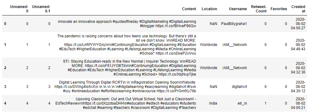

At a first glance, we can see that there are 202.645 tweets including the content, location, username, Retweet count, Favorites count, and the creation time features in the DataFrame. There are also some missing values in the Location column. We’ll deal with them in the next step.

乍一看，我们可以看到有202.645条Tweet，包括内容，位置，用户名，Retweet计数，收藏夹计数以及DataFrame中的创建时间功能。 在位置列中也缺少一些值。 我们将在下一步中处理它们。

2.预处理和清洁 (2. Preprocessing and Cleaning)

According to the information above, Unnamed: 0 and Unnamed: 0.1 columns are not informative to us so we’ll drop them out. The data type of Created at column also should be datetime. As well as we need to get rid of duplicated tweets if there are some.

根据上面的信息，“ 未命名：0”和“ 未命名：0.1”列对我们没有帮助，因此我们将其删除。 Created at列的数据类型也应为datetime。 同样，如果有的话，我们需要消除重复的推文。

# We do not need first two columns. Let's drop them out.
tweets_raw.drop(columns=["Unnamed: 0", "Unnamed: 0.1"], axis=1, inplace=True)# Drop duplicated rows
tweets_raw.drop_duplicates(inplace=True)# Created at column's type should be datatime
tweets_raw["Created at"] = pd.to_datetime(tweets_raw["Created at"])# Print the info again
print(tweets_raw.info())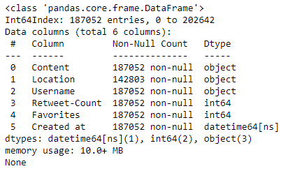

The tweets count has been reduced to 187.052 (There were 15.593 duplicated rows). “Created at” column’s data type is also changed to datatime64[ns].

发推数已减少至187.052 (重复的行数为15.593 )。 “ Created at”列的数据类型也更改为datatime64 [ns] 。

Now, let’s tidy the tweets’ contents up. We need to get rid of stopwords, punctuation, hashtags, mentions, links, and one or two-letter words. As well as we need to tokenize the tweets.

现在，让我们整理推文的内容。 我们需要去除停用词 ， 标点符号 ， 主题标签 ， 提及 ， 链接以及一个或两个字母的单词 。 以及我们需要标记这些推文。

Tokenization is the splitting of a sentence into words and punctuation marks. The sentence “This is an example.” can be tokenized like [“This”, “is”, “an”, “example”, “.”]

标记化是将句子分为单词和标点符号。 句子“这是一个例子。” 可以像[“ This”，“ is”，“ an”，“ example”，“。”]这样标记

Stopwords are the words that are commonly used and they don’t contribute to the meaning of a sentence such as “a”, “an”, “the”, “on”, “in” and so forth.

停用词是常用的词，对诸如“一个”，“一个”，“该”，“在”，“在”等中的句子的意义没有帮助。

Lemmatization is the process of reducing a word to its root form. This root form called a lemma. For example, the lemma of words running runs, and ran is run

合法化 是将单词还原为词根形式的过程。 这种根形式称为引理 。 例如， 运行 运行的话引理， 跑 运行

Let’s define a function to do all of these operations.

让我们定义一个函数来执行所有这些操作。

After the function call, our Processed column will be like the following. You see that the tweets are tokenized and they do not contain stopwords, hashtags, links, and one or two-letter words. We also applied the lemmatization operation on them.

函数调用后，“已处理”列将如下所示。 您会看到这些推文已被标记化，并且它们不包含停用词，＃标签，链接以及一个或两个字母的词。 我们还对它们应用了词形化操作。

We got what we want. Do not worry about words such as learning, online, education, etc. We will deal with them later.

我们得到了我们想要的。 不用担心诸如学习 ， 在线 ， 教育等词语。我们稍后将处理它们。

Tweet lengths and number of words in the tweets might be also interesting in the exploratory data analysis. Let’s get them!

在探索性数据分析中，推文中的推文长度和单词数可能也很有趣。 让我们得到它们！

# Get the tweet lengths
tweets_raw["Length"] = tweets_raw["Content"].str.len()# Get the number of words in tweets
tweets_raw["Words"] = tweets_raw["Content"].str.split().str.len()# Display the new columns
display(tweets_raw[["Length", "Words"]])

Notice that we did not use the Processed tweets.

请注意，我们没有使用已处理的推文。

What about the locations?

地点呢？

When we called the info function of tweets_raw DataFrame, we saw that there were some missing values in the “Location” columns. The missing values are indicated as NaN. We’ll fill the missing values with the “unknown” tag.

当我们调用tweets_raw DataFrame的info函数时 ，我们发现“位置”列中缺少一些值。 缺失值表示为NaN 。 我们将使用“未知”标签填充缺失的值。

# Fill the missing values with unknown tag
tweets_raw["Location"].fillna("unknown", inplace=True)

How many unique locations we have?

我们有几个独特的位置？

# Print the unique locations and number of unique locations
print("Unique Values:",tweets_raw["Location"].unique())
print("Unique Value count:",len(tweets_raw["Location"].unique()))

The outputs show us the location information is messy. There are 37.119 unique locations. We need to group them by country. To achieve this, we will use the pycountry package in python. If you are interested, you can find further information here.

输出显示位置信息混乱。 有37.119个唯一位置。 我们需要按国家对它们进行分组。 为此，我们将在python中使用pycountry包。 如果您有兴趣，可以在此处找到更多信息。

Let’s define a function called get_countries which returns the country codes of the given locations.

让我们定义一个名为get_countries的函数，该函数返回给定位置的国家/地区代码。

It worked! Now we have 156 unique country codes. We will use them for the exploratory data analysis part.

有效！ 现在我们有156个唯一的国家/地区代码。 我们将在探索性数据分析部分中使用它们。

Now it’s time to vectorize the tweets. We’ll use tf-idf (term frequency-inverse document term frequency) vectorization.

现在是时候将推文矢量化了。 我们将使用tf-idf(术语频率-反文档术语频率)矢量化。

Tf-idf (Term Frequency — Inverse Term Frequency) is a statistical concept to be used to get the frequency of words in the corpus. We’ll use scikit-learn’s TfidfVectorizer. The vectorizer will calculate the weight of each word in the corpus and will return a tf-idf matrix. You can find further information here

Tf-idf(术语频率-术语频率的倒数)是一种统计概念，用于获取语料库中单词的频率。 我们将使用scikit-learn的TfidfVectorizer 。 矢量化器将计算语料库中每个单词的权重，并返回tf-idf矩阵。 您可以在此处找到更多信息

td = Term frequency (number of occurrences each i in j)df = Document frequencyN = Number of documentsw = tf-idf weight for each i and j (document).

td =术语频率(j中每个i中出现的次数) df =文档频率N =文档数w =每个i和j (文档)的tf-idf权重。

We are going to select only the top 5000 words for tf-idf vectorization due to memory constraints. You can experiment with more by using other approaches like hashing.

由于内存限制，我们将仅选择tf-idf矢量化的前5000个字 。 您可以使用其他方法(例如哈希)进行更多试验。

# Create our contextual stop words
tfidf_stops = ["online","class","course","learning","learn",\
"teach","teaching","distance","distancelearning","education",\
"teacher","student","grade","classes","computer","onlineeducation",\ "onlinelearning", "school", "students","class","virtual","eschool",\ "virtuallearning", "educated", "educates", "teaches", "studies",\ "study", "semester", "elearning","teachers", "lecturer", "lecture",\ "amp","academic", "admission", "academician", "account", "action" \
"add", "app", "announcement", "application", "adult", "classroom", "system", "video", "essay", "homework","work","assignment","paper",\ "get", "math", "project", "science", "physics", "lesson","courses",\ "assignments", "know", "instruction","email", "discussion","home",\ "college","exam""use","fall","term","proposal","one","review",\
"proposal", "calculus", "search", "research", "algebra"]# Initialize a Tf-idf Vectorizer
vectorizer = TfidfVectorizer(max_features=5000, stop_words= tfidf_stops)# Fit and transform the vectorizer
tfidf_matrix = vectorizer.fit_transform(tweets_processed["Processed"])# Let's see what we have
display(tfidf_matrix)# Create a DataFrame for tf-idf vectors and display the first rows
tfidf_df = pd.DataFrame(tfidf_matrix.toarray(), columns= vectorizer.get_feature_names())
display(tfidf_df.head())

It returned us a sparse matrix. You can look at its content below.

它给我们返回了一个稀疏矩阵。 您可以在下面查看其内容。

PAfter all, we save the new DataFrame as a CSV file to use later without performing whole operations again.

P毕竟，我们将新的DataFrame保存为CSV文件，以供以后使用，而无需再次执行整个操作。

# Save the processed data as a csv file
tweets_raw.to_csv("tweets_processed.csv")

3.探索性数据分析 (3. Exploratory Data Analysis)

Exploratory data analysis is an indispensable part of data science projects. We can build our models as long as we understand what our data tell us.

探索性数据分析是数据科学项目必不可少的部分。 只要我们了解数据告诉我们的内容，便可以构建模型。

# Load the processed DataFrame
tweets_processed = pd.read_csv("tweets_processed.csv", parse_dates=["Created at"])

First of all, let’s look at the oldest and the newest tweets creation time in our data set.

首先，让我们看一下数据集中最早的和最新的推文创建时间。

# Print the minimum datetime
print("Since:",tweets_processed["Created at"].min())# Print the maximum datetime
print("Until",tweets_processed["Created at"].max())

The tweets have been created between 23 July and 14 August 2020. What about the creation hours?

这些推文是在2020年7月23日至8月14日之间创建的。创建时间如何？

# Set the seaborn style
sns.set()# Plot the histogram of hours
sns.distplot(tweets_processed["Created at"].dt.hour, bins=24)
plt.title("Hourly Distribution of Tweets")
plt.show()

The histogram demonstrates that most of the tweets are created between 12 am-17 pm in a day. The most popular hour is about 15 pm.

直方图表明，大多数推文是一天中的12点至17点之间创建的。 最受欢迎的时间是下午15点左右。

Let’s look at the locations that we have already processed.

让我们看一下我们已经处理过的位置。

# Print the value counts of Country column
print(tweets_processed["Country"].value_counts())

Apparently, the locations will be noninformative for us because we have 169.734 unknown locations. But we can still check the top tweeting countries.

显然，这些位置对我们而言是无意义的，因为我们有169.734个未知位置。 但是，我们仍然可以查看发帖最多的国家/地区。

According to the bar plot above, United States, United Kingdom, and India are the top 3 countries in our dataset.

根据上面的条形图， 美国 ， 英国和印度是我们数据集中的前3个国家/地区。

Now, let’s look at the most popular tweets (in terms of retweets and favorites).

现在，让我们看一下最受欢迎的推文(在转发和收藏夹方面)。

# Display the most popular tweets
display(tweets_processed.sort_values(by=["Favorites","Retweet-Count", ], axis=0, ascending=False)[["Content","Retweet-Count","Favorites"]].head(20))

Popular tweets, click on the image to see better

热门推文，请点击图片查看更好

The frequent words in the tweets can also tell us a lot. Let’s get them from our Tf-idf matrix.

推文中的常用词也可以告诉我们很多东西。 让我们从Tf-idf矩阵中获取它们。

# Create a new DataFrame called frequencies
frequencies = pd.DataFrame(tfidf_matrix.sum(axis=0).T,index=vectorizer.get_feature_names(),columns=['total frequency'])# Display the most 20 frequent words
display(frequencies.sort_values(by='total frequency',ascending=False).head(20))

Word clouds would be nicer.

词云会更好。

Wordcloud, image by author

Wordcloud，作者提供的图片

Apparently, people talk about “payment”. “Help” is one of the most frequent words. We can say that people are looking for help a lot :)

显然，人们谈论“付款” 。 “帮助”是最常用的词之一。 我们可以说人们在寻求帮助很多：)

4.情绪分析 (4. Sentiment Analysis)

After preprocessing and EDA, we can finally focus on our main aim in this project. We are going to calculate the tweets’ sentimental features such as polarity and subjectivity by using TextBlob. It gives us these values by using the predefined word scores. You can check the documentation for more information.

经过预处理和EDA，我们最终可以专注于该项目的主要目标。 我们将使用TextBlob计算推文的情感特征，例如极性和主观性 。 它通过使用预定义的单词分数为我们提供了这些值。 您可以查看文档以获取更多信息。

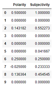
polarity is a value changes between -1 to 1. It shows us how positive or negative the sentence given is.

极性是在-1 到 1之间变化的值。 它向我们展示了给出的句子是正面还是负面 。

subjectivity is another value changes between 0 to 1 which shows us whether the sentence is about a fact or opinion (objective or subjective).

主观性是另一个介于0到1之间的值，它向我们显示了句子是关于事实还是观点(客观还是主观)。

Let’s calculate the polarity and subjectivity scores with TextBlob

让我们用TextBlob计算极性和主观性得分

We need to classify the polarities as positive, neutral, and negative.

我们需要将极性分为正极性，中性和负极性。

We can also count them up like the following.

我们还可以像下面这样对它们进行计数。

# Print the value counts of the Label column
print(tweets_processed["Label"].value_counts())

The results are different than what I expected. Positive tweets are significantly more than negative ones.

结果与我预期的不同。 正面的推文比负面的要多得多。

We tagged the tweets as positive, neutral, and negative so far. Let’s go over our findings deeply. I will start with label counts.

到目前为止，我们将这些推文标记为正面，中性和负面。 让我们深入研究我们的发现。 我将从标签数量开始。

# Change the datatype as "category"
tweets_processed["Label"] = tweets_processed["Label"].astype("category")# Visualize the Label counts
sns.countplot(tweets_processed["Label"])
plt.title("Label Counts")
plt.show()# Visualize the Polarity scores
plt.figure(figsize = (10, 10)) 
sns.scatterplot(x="Polarity", y="Subjectivity", hue="Label", data=tweets_processed)
plt.title("Subjectivity vs Polarity")
plt.show()

Since the lexicon-based analysis is not always reliable, we have to check the results manually. Let’s see the popular (in terms of retweets and favorites) tweets that have the highest/lowest polarity scores.

由于基于词典的分析并不总是可靠的，因此我们必须手动检查结果。 让我们看看具有最高/最低极性分数的流行(就转发和收藏而言)。

# Display the positive tweets
display(tweets_processed.sort_values(by=["Polarity", "Retweet-Count", "Favorites"], axis=0, ascending=False)[["Content","Retweet-Count","Favorites","Polarity"]].head(20))# Display the negative tweets
display(tweets_processed.sort_values(by=["Polarity", "Retweet-Count", "Favorites"], axis=0, ascending=[True, False, False])[["Content","Retweet-Count","Favorites","Polarity"]].head(20))

Positive tweets, click on the image to see better

正面推文，点击图片可查看更好

Negative tweets, , click on the image to see better

负面推文，，点击图片查看更好

According to the results above, TextBlob has done its job correctly! We can make word clouds for each label as we did above. To do this, I will define a function. The function will take a DataFrame and a label as arguments and vectorized the Processed tweets with tf-idf vectorizer. Finally, it will make the word clouds for us. We will only look at the most popular 50 tweets because of the computational constraints. You can try with more data.

根据上面的结果，TextBlob正确完成了工作！ 我们可以像上面一样为每个标签制作词云。 为此，我将定义一个函数。 该函数将使用一个DataFrame和一个标签作为参数，并使用tf-idf矢量化器对已处理的 tweet进行矢量化。 最终，这将使我们感到困惑。 由于计算限制，我们将仅关注最受欢迎的50条推文。 您可以尝试使用更多数据。

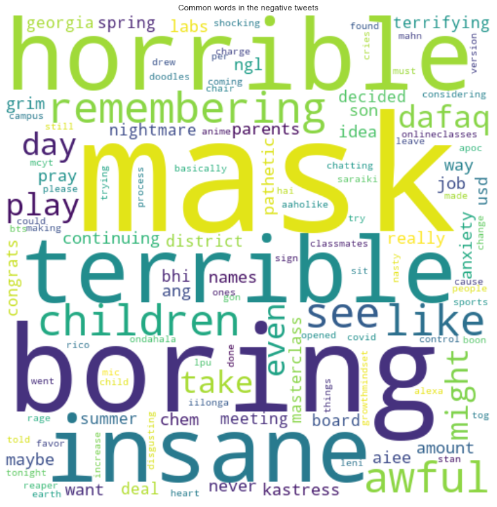
Apparently, people whose tweets are negative find distance learning is boring, horrible, and terrible. On the other hand, some people like options for distance learning.

显然，推文为负面的人们发现远程学习很无聊，可怕和可怕。 另一方面，有些人喜欢远程学习的选择。

Let’s look at the positive and negative tweet counts by country.

让我们看一下按国家划分的正面和负面推文计数。

Is there any relationship between the time and tweets’ polarities?

时间和推文极性之间是否有任何关系？

positive = tweets_processed.loc[tweets_processed.Label=="Positive"]["Created at"].dt.hour
negative = tweets_processed.loc[tweets_processed.Label=="Negative"]["Created at"].dt.hourplt.hist(positive, alpha=0.5, bins=24, label="Positive", density=True)
plt.hist(negative, alpha=0.5, bins=24, label="Negative", density=True)
plt.xlabel("Hour")
plt.ylabel("PDF")
plt.title("Hourly Distribution of Tweets")
plt.legend(loc='upper right')
plt.show()

The histogram above demonstrates that there is no relationship between the time and tweets’ polarities.

上面的直方图表明时间和推文极性之间没有关系。

I want to finish my exploration here to keep this story short.

我想在这里结束我的探索，以使这个故事简短。

5.建立机器学习模型 (5. Build a Machine Learning Model)

We have labeled the tweets according to their polarity scores. Let’s build a Machine Learning model by using a Multinomial Naive Bayes Classifier. We will use our tf-idf vectors as the features and the labels as the target.

我们已经根据推文的极性得分为其打了标签。 让我们使用多项朴素贝叶斯分类器构建机器学习模型。 我们将使用tf-idf向量作为特征，并使用标签作为目标。

# Encode the labels
le = LabelEncoder()
tweets_processed["Label_enc"] = le.fit_transform(tweets_processed["Label"])# Display the encoded labels
display(tweets_processed[["Label_enc"]].head())

We have encoded the labels.

我们已经对标签进行了编码。

“Positive” = 2

“正数” = 2

“Neutral” = 1

“中立” = 1

“Negative” = 0

“负数” = 0

# Select the features and the target
X = tweets_processed['Processed']
y = tweets_processed["Label_enc"]

Now, we need to split our data into train and test sets. We’ll use the stratify parameter of train_test_split since our data is unbalanced.

现在，我们需要将数据拆分为训练集和测试集。 因为我们的数据是不平衡的，我们将使用train_test_split的分层参数。

X_train, X_test, y_train, y_test = train_test_split(X, y, test_size=0.2, random_state=34, stratify=y)

Now, we can create our model. Since our earlier tf-idf vectorizer fit by the entire dataset, we have to initialize a new one. Otherwise, our model can learn by the test set.

现在，我们可以创建模型。 由于我们较早的tf-idf矢量化器适合整个数据集，因此我们必须初始化一个新的tf-idf矢量化器。 否则，我们的模型可以通过测试集学习。

# Create the tf-idf vectorizer
model_vectorizer = TfidfVectorizer()# First fit the vectorizer with our training set
tfidf_train = vectorizer.fit_transform(X_train)# Now we can fit our test data with the same vectorizer
tfidf_test = vectorizer.transform(X_test)# Initialize the Bernoulli Naive Bayes classifier
nb = BernoulliNB()# Fit the model
nb.fit(tfidf_train, y_train)# Print the accuracy score
best_accuracy = cross_val_score(nb, tfidf_test, y_test, cv=10, scoring='accuracy').max()
print("Accuracy:",best_accuracy)

Although we did not do any hyperparameter tuning, the accuracy is not bad. Let’s look at the confusion matrix and classification report.

尽管我们没有进行任何超参数调整，但准确性还不错。 让我们看看混淆矩阵和分类报告。

# Predict the labels
y_pred = nb.predict(tfidf_test)# Print the Confusion Matrix
cm = confusion_matrix(y_test, y_pred)
print("Confusion Matrix\n")
print(cm)# Print the Classification Report
cr = classification_report(y_test, y_pred)
print("\n\nClassification Report\n")
print(cr)

There is still a lot to do for improving the model’s performance on negative tweets but I keep it for another story :)

要改善模型在负面推文上的性能，还有很多工作要做，但我会继续讲另一个故事:)

Finally, we can save the model to use later.

最后，我们可以保存模型以供以后使用。

# Save the model
pickle.dump(nb, open("model.pkl", 'wb'))

摘要 (Summary)

In summary, let’s remember what we did together. Firstly, we have collected the Tweets about distance learning by using Twitter API and the tweepy library. After that we applied common preprocessing steps on them such as tokenization, lemmatization, removing stopwords, and so forth. We explored the data by using summary statistics and visualization tools. After all, we used TextBlob to get polarity scores of the tweets and interpreted our findings. Consequently, we found that in our dataset most of the tweets have positive opinions about distance learning. Do not forget the fact that we only used a lexicon-based approach which is not very reliable. I hope this story will be helpful for you to understand the sentiment analysis of tweets.

总而言之，让我们记住我们一起做的事情。 首先，我们使用Twitter API和tweepy库收集了有关远程学习的推文。 之后，我们对它们应用了通用的预处理步骤，例如标记化，词形化，去除停用词等。 我们使用摘要统计信息和可视化工具探索了数据。 毕竟，我们使用TextBlob来获取推文的极性得分并解释我们的发现。 因此，我们发现在我们的数据集中，大多数推文对远程学习都持积极态度。 不要忘记我们只使用了基于词典的方法，这种方法不是很可靠的事实。 希望这个故事对您了解推文的情绪分析有所帮助。

[1] (Tutorial) simplifying sentiment analysis in Python. (n.d.). DataCamp Community. https://www.datacamp.com/community/tutorials/simplifying-sentiment-analysis-python

[1] (教程)简化Python中的情感分析 。 (nd)。 DataCamp社区。 https://www.datacamp.com/community/tutorials/simplifying-sentiment-analysis-python

[2] Lee, J. (2020, May 19). Twitter sentiment analysis | NLP | Text analytics. Medium. https://towardsdatascience.com/twitter-sentiment-analysis-nlp-text-analytics-b7b296d71fce

[2] Lee，J.(2020年，5月19日)。 Twitter情绪分析| NLP | 文本分析 。 中。 https://towardsdatascience.com/twitter-sentiment-analysis-nlp-text-analytics-b7b296d71fce

[3] Li, C. (2019, September 20). Real-time Twitter sentiment analysis for brand improvement and topic tracking (Chapter 1/3). Medium. https://towardsdatascience.com/real-time-twitter-sentiment-analysis-for-brand-improvement-and-topic-tracking-chapter-1-3-e02f7652d8ff

[3] Li，C.(2019年9月20日)。 实时Twitter情绪分析，用于品牌改进和主题跟踪(第1/3章) 。 中。 https://towardsdatascience.com/real-time-twitter-sentiment-analysis-for-brand-improvement-and-topic-tracking-chapter-1-3-e02f7652d8ff

[4] Randerson112358. (2020, July 18). How to do sentiment analysis on a Twitter account in Python. Medium. https://medium.com/better-programming/twitter-sentiment-analysis-15d8892c0082

[4] Randerson112358。 (2020年，7月18日)。 如何在Python中对Twitter帐户进行情感分析 。 中。 https://medium.com/better-programming/twitter-sentiment-analysis-15d8892c0082

[5] Stemming and Lemmatization in Python. (n.d.). DataCamp Community. https://www.datacamp.com/community/tutorials/stemming-lemmatization-python

[5] Python中的词干和词法化 。 (nd)。 DataCamp社区。 https://www.datacamp.com/community/tutorials/stemming-lemmatization-python

翻译自: https://towardsdatascience.com/sentiment-analysis-on-the-tweets-about-distance-learning-with-textblob-cc73702b48bc

textblob 情感分析