可视化新工具 —— HoloViews

觉得绘制数据像是迷宫而不是地图吗？那么，HoloViews来拯救我们了！它就像是Python中的一种神奇工具，让处理数据变得轻而易举。想象一下，我们可以让我们的数据自己展示，让我们专注于有趣的事情，而不是头疼于绘图的问题。HoloViews保持简单 - 只需几行代码，我们就可以开始了。告别令人困惑的图表，迎接不费吹灰之力地探索我们的数据。

为什么选择HoloViews？

我们可能会想，Python已经有了像numpy、pandas以及绘图工具bokeh和matplotlib这样的强大工具，为什么要选择HoloViews呢？HoloViews不仅仅是关于绘图；它关乎在瞬间理解我们的数据。它能够平滑地将我们的数据与其可视化部分连接起来。

与通常分别处理数据和绘图的常规程序不同，HoloViews将它们捆绑在一起并附加额外的信息。这样，我们的原始数据和其可视化版本始终保持同步。这可能与我们习惯的方式有些不同，但本指南将引导我们逐步了解。使用HoloViews，我们只需简要描述我们的数据，添加一些额外的细节，咔擦！由于Bokeh或Matplotlib等库的存在，即刻自动生成可视化。不再烦扰；我们的数据发展，视觉效果也随之而来。

安装

安装和运行HoloViews非常简单。它与在Linux、Windows或Mac上的Python 3兼容，并且与Jupyter Notebook和JupyterLab协同工作。最简单的方法是使用Anaconda或Miniconda通过conda命令：

#使用conda安装HoloViews和Bokeh
conda install -c pyviz holoviews bokeh

这个命令不仅会安装HoloViews，还会获取与之搭配得很好的常用包。HoloViews本身只需要Numpy、Pandas和Param来完成它的任务。如果你不使用Conda，可以从GitHub获取HoloViews，并按照以下步骤进行安装。

#从GitHub克隆HoloViews
git clone git://github.com/holoviz/holoviews.git
#进入HoloViews目录
cd holoviews
#安装HoloViews
pip install -e .

初学者指南

为了亲身体验HoloViews，让我们使用一组与纽约市交通相关的数据集。我们将从加载的CSV文件中开始，该文件包含有关地铁站的信息：

#Import necessary librariesimport pandas as pd # For data manipulation and analysis
import numpy as np # For numerical operations
import holoviews as hv # For interactive data visualization
from holoviews import opts # For setting plotting options
hv.extension('bokeh') # Activate Bokeh as the plotting extension

在这里，我们确保numpy和pandas准备就绪。始终将HoloViews导入为hv。在导入HoloViews后，运行hv.extension('bokeh')加载Bokeh绘图扩展，使得使用Bokeh进行可视化成为可能。现在，让我们深入研究地铁数据：

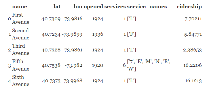
# Load subway station information from a CSV filestation_info = pd.read_csv('station_info.csv')
Display the first few rows of the station_info dataframestation_info.head()

该表包括地铁站的详细信息，如名称、纬度、经度、开放年份、服务、服务名称和乘客数量。

现在，让我们用散点图可视化数据，探索乘客数量与服务数量的变化：

# Create a scatter plot using HoloViews
# where 'services' is on the x-axis and 'ridership' is on the y-axis
scatter = hv.Scatter(station_info, 'services', 'ridership')
scatter

在这里，scatter是一个HoloViews对象，还不是图表。它会自动使用Bokeh进行可视化。HoloViews提供各种元素类型；在这种情况下，scatter是对数据框的包装器，将 'services' 和 'ridership' 列理解为维度。通过打印确认它是一个对象：

#打印关于散点图对象的信息
print(scatter)
```plaintext
######### 输出   #############
:Scatter [services]   (ridership)
######### 输出   #############

现在，让我们超越单一图表。我们可以创建组合布局，例如将散点图与直方图结合起来：

#创建组合布局
#通过将散点图与直方图结合
layout = scatter + hv.Histogram(np.histogram(station_info['opened'], bins=24), kdims=['opened'])
layout

使用+运算符，形成了一个新的Layout对象。它包含散点图和一个直方图，显示自1900年以来曼哈顿地铁站的开放情况。记住，布局不是一个图表，而是一个独立的对象：

# 打印关于布局对象的信息
print(layout)
```plaintext
################ 输出       ################
:Layout
.Scatter.I   :Scatter   [services]   (ridership)
.Histogram.I :Histogram   [opened]   (Frequency)
################ 输出       ################

我们可以通过创建一个交互式的HoloMap，其中包含表示一天中特定小时的出租车下车点的图像字典，轻松探索和可视化数据。

# 步骤1：为每天的每个小时生成图像字典
image_dictionary = {
int(hour): hv.Image(arr, ['lon', 'lat'], bounds=bounds)
for hour, arr in taxi_dropoffs.items()
}
# 步骤2：创建键维度的列表（'Hour'）
key_dimensions_list = ['Hour']
# 步骤3：使用生成的字典和键维度创建交互式HoloMap
holo_map = hv.HoloMap(image_dictionary, kdims=key_dimensions_list)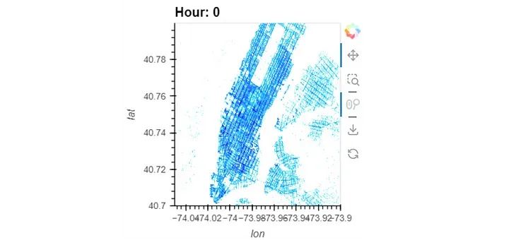

处理实时数据

实时数据有很多形式，如实时财务数据或持续的科学测量。现在，让我们讨论由两个简单方程创建的简单路径：

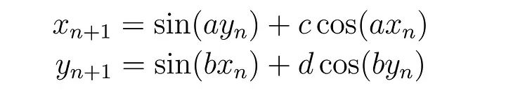
现在，让我们编写一个Python函数，从初始位置（x0, y0）开始迭代给定的Clifford方程：

# Import the NumPy library as np for numerical operations
import numpy as np


# Define a Python function named clifford_equation with parameters a, b, c, d, x0, and y0
def clifford_equation(a, b, c, d, x0, y0):
    # Initialize variables xn and yn with the initial positions x0 and y0
    xn, yn = x0, y0


    # Create a list to store the coordinates, starting with the initial position
    coords = [(x0, y0)]


    # Iterate through the equations for 10,000 steps
    for i in range(10000):
        # Calculate the next x-coordinate using the Clifford equations
        x_n1 = np.sin(a * yn) + c * np.cos(a * xn)
        
        # Calculate the next y-coordinate using the Clifford equations
        y_n1 = np.sin(b * xn) + d * np.cos(b * yn)
        
        # Update xn and yn with the newly calculated coordinates
        xn, yn = x_n1, y_n1
        
        # Append the current coordinates to the list
        coords.append((xn, yn))


    # Return the list of coordinates
    return coords

当我们执行此函数时，它目前会生成一个包含10,000个元组的列表。为了更好地理解这些数据，我们可以为Curve和Points元素建立适当的可视化默认值：

# Import necessary components from HoloViews
from holoviews import opts
import holoviews as hv


# Set default visual options for Curve and Points elements
opts.defaults(
    opts.Curve(color='black'),  # Set Curve color to black
    opts.Points(color='red', alpha=0.1, width=400, height=400)  # Set Points color to red, adjust alpha, width, and height
)

现在，我们可以轻松地将我们的 Clifford 函数的输出作为 Points 元素的输入。这简化了定义一个函数的过程，当调用该函数时，它会为我们提供一个可视化。

# Define a function that creates a HoloViews Points element for the Clifford attractor
def clifford_attractor(a, b, c, d):
    return hv.Points(clifford_equation(a, b, c, d, x0=0, y0=0))


# View the output for specific values of a, b, c, d, starting from the origin
clifford_attractor(a=-1.5, b=1.5, c=1, d=0.75)

这个特定的HoloViews元素捕捉了选定的四个值的快照。然而，我们的目标是直接与四维参数空间进行交互。尽管这个参数空间的大小使得计算所有可能的组合变得不切实际，但我们的目标是实现直接的交互。

·  END  ·

HAPPY LIFE

本文仅供学习交流使用，如有侵权请联系作者删除