分类模型性能评估及调参

---

转载来源：datawhale-集成学习
参考资料：

• 内容思路：https://zhuanlan.zhihu.com/p/140040705
• 归一化：https://blog.csdn.net/wzyaiwl/article/details/90549391
• 支持向量机（分类）：http://ihoge.cn/2018/SVWSVC.html

---

1. GridSearchCV流程

    1.1 人工设定参数
    1.2 排列组合并遍历比较结果
   

2. RandomSearchCV搜索流程

    2.1 对于搜索范围是distribution的超参数，根据给定的distribution随机采样；
    2.2 对于搜索范围是list的超参数，在给定的list中等概率采样；
    2.3 对a、b两步中得到的n_iter组采样结果，进行遍历。
    	（补充）如果给定的搜索范围均为list，则不放回抽样n_iter次。
   

---

代码实现、调试及各变量

# 导入工具包
import numpy as np
import pandas as pd
import matplotlib.pyplot as plt
%matplotlib inline
plt.style.use("ggplot")
import warnings
warnings.filterwarnings("ignore")

# 使用网格搜索进行超参数调优：
# 方式1：网格搜索GridSearchCV()

from sklearn.pipeline import make_pipeline     			# 管道函数
from sklearn.model_selection import GridSearchCV		# 网格搜索
from sklearn.svm import SVC								# 导入分类支持向量机
import time												# 导入时间函数用于计时

start_time = time.time() 								# 设置开始时间
pipe_svc = make_pipeline(								# 构建管道封装工作流
						StandardScaler(), 				# 设置归一化
						SVC(random_state=1)				# 设置随机种子数
						)
param_range = [0.0001,0.001,0.01,0.1,1.0,10.0,100.0,1000.0]
param_grid = [	{'svc__C':param_range,'svc__kernel':['linear']},
				{'svc__C':param_range,'svc__gamma':param_range,'svc__kernel':['rbf']}]
				
gs = GridSearchCV(	estimator=pipe_svc,
					param_grid=param_grid,
					scoring='accuracy',
					cv=10,n_jobs=-1)
gs = gs.fit(X,y)
end_time = time.time()
print("网格搜索经历时间：%.3f S" % float(end_time-start_time))
print(gs.best_score_)
print(gs.best_params_)

网格搜索经历时间：6.728 S
0.93
{'svc__C': 10.0, 'svc__gamma': 1.0, 'svc__kernel': 'rbf'}

________________________________
SVM：support vector machine 
SVR：support vector regression
SVC：support vector classic
________________________________

1. StandardScaler()：设置归一化

	1.1 归一化后加快了梯度下降求最优解的速度；
		
		如果机器学习模型使用梯度下降法求最优解时，归一化往往非常有必要，否则很难收敛甚至不能收敛
		
	1.2 归一化有可能提高精度
		
			一些分类器需要计算样本之间的距离（如欧氏距离），例如KNN。
		如果一个特征值域范围非常大，那么距离计算就主要取决于这个特征，从而与实际情况相悖，
		比如这时实际情况是值域范围小的特征更重要
		
2. svm.SVC分类器简介：

	2.01 C：C-SVC的惩罚参数C?默认值是1.0
		
		C越大，相当于惩罚松弛变量，希望松弛变量接近0，即对误分类的惩罚增大，
	趋向于对训练集全分对的情况，这样对训练集测试时准确率很高，但泛化能力弱。
		C值小，对误分类的惩罚减小，允许容错，将他们当成噪声点，泛化能力较强。
		
	2.02 kernel ：核函数，默认是rbf，可以是'linear','poly','rbf'
	
		- liner：线性核函数：u'v
		- poly：多项式核函数：(gamma*u'*v + coef0)^degree
		- rbf：RBF高斯核函数：exp(-gamma|u-v|^2)

	2.03 degree ：多项式poly函数的维度，默认是3，选择其他核函数时会被忽略。

	2.03 gamma ： ‘rbf’,‘poly’ 和‘sigmoid’的核函数参数。默认是’auto’，则会选择1/n_features

	2.05 coef0 ：核函数的常数项。对于‘poly’和 ‘sigmoid’有用。

	2.06 probability ：是否采用概率估计？.默认为False

	2.07 shrinking ：是否采用shrinking heuristic方法，默认为true

	2.08 tol ：停止训练的误差值大小，默认为1e-3

	2.09 cache_size ：核函数cache缓存大小，默认为200

	2.10 class_weight ：类别的权重，字典形式传递。设置第几类的参数C为weight*C(C-SVC中的C)

	2.11 verbose ：允许冗余输出？

	2.12 max_iter ：最大迭代次数。-1为无限制。

	2.13 decision_function_shape ：‘ovo’, ‘ovr’ or None, default=None3

	2.14 random_state ：数据洗牌时的种子值，int值
		使每次构建的随机分类一样
		https://www.zhihu.com/question/56315846/answer/148520029
		
3.  常用参数解读
	3.1 estimator：所使用的分类器，如
		estimator=RandomForestClassifier(	min_samples_split=100,
											min_samples_leaf=20,
											max_depth=8,
											max_features='sqrt',
											random_state=10), 
		并且传入除需要确定最佳的参数之外的其他参数。
		每一个分类器都需要一个scoring参数，或者score方法。

	3.2 param_grid：值为字典或者列表，即需要最优化的参数的取值，
		param_grid =param_test1
		param_test1 = {'n_estimators':range(10,71,10)}。

	3.3 scoring :准确度评价标准，默认None,这时需要使用score函数；或者如scoring=’roc_auc’，
		根据所选模型不同，评价准则不同。字符串（函数名），或是可调用对象，需要其函数签名形如：scorer(estimator, X, y)；
		如果是None，则使用estimator的误差估计函数。下文表格中详细指定了score可取的值和函数形式。

	3.4 cv :交叉验证参数，默认None，使用三折交叉验证。
		指定fold数量，默认为3，也可以是yield训练/测试数据的生成器。也可是是诸如StratifiedKFold(n_splits=10)这样的类对象。

	3.5 refit :默认为True,程序将会以交叉验证训练集得到的最佳参数，重新对所有可用的训练集与开发集进行，
		作为最终用于性能评估的最佳模型参数。即在搜索参数结束后，用最佳参数结果再次fit一遍全部数据集。

	3.6 iid:默认True,为True时，默认为各个样本fold概率分布一致，误差估计为所有样本之和，而非各个fold的平均。

	3.7 verbose：日志冗长度，int：冗长度，0：不输出训练过程，1：偶尔输出，>1：对每个子模型都输出。

	3.8 n_jobs: 并行数，int：个数,-1：跟CPU核数一致, 1:默认值。

	3.9 pre_dispatch：指定总共分发的并行任务数。当n_jobs大于1时，数据将在每个运行点进行复制，这可能导致OOM，（）
	而设置pre_dispatch参数，则可以预先划分总共的job数量，使数据最多被复制pre_dispatch次

# 方式2：随机网格搜索RandomizedSearchCV()
from sklearn.model_selection import RandomizedSearchCV				# 导入随机搜索
from sklearn.svm import SVC											
import time

start_time = time.time()
pipe_svc = make_pipeline(StandardScaler(),SVC(random_state=1))		# 构建分类器
param_range = [0.0001,0.001,0.01,0.1,1.0,10.0,100.0,1000.0]
param_grid = [	{'svc__C':param_range,'svc__kernel':['linear']},	
				{'svc__C':param_range,'svc__gamma':param_range,'svc__kernel':['rbf']}]
# param_grid = [{'svc__C':param_range,'svc__kernel':['linear','rbf'],'svc__gamma':param_range}]

gs = RandomizedSearchCV(estimator=pipe_svc, 						# 选择分类器
						param_distributions=param_grid,				# 设定搜索值范围
						scoring='accuracy',						 
						cv=10,
						n_jobs=-1)
gs = gs.fit(X,y)
end_time = time.time()
print("随机网格搜索经历时间：%.3f S" % float(end_time-start_time))
print(gs.best_score_)
print(gs.best_params_)

随机网格搜索经历时间：5.664 S
0.9
{'svc__kernel': 'rbf', 'svc__gamma': 0.01, 'svc__C': 1000.0}

---

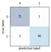
当类别为两类时，可以绘制混淆矩阵与ROC曲线

混淆矩阵原理：https://zhuanlan.zhihu.com/p/46204175

# 混淆矩阵：
# 加载数据
df = pd.read_csv("http://archive.ics.uci.edu/ml/machine-learning-databases/breast-cancer-wisconsin/wdbc.data",header=None)
'''
乳腺癌数据集：569个恶性和良性肿瘤细胞的样本，M为恶性，B为良性
'''
# 做基本的数据预处理
from sklearn.preprocessing import LabelEncoder

X = df.iloc[:,2:].values
y = df.iloc[:,1].values
le = LabelEncoder()    								#将M-B等字符串编码成计算机能识别的0-1
y = le.fit_transform(y)
le.transform(['M','B'])

# 数据切分8:2
from sklearn.model_selection import train_test_split

X_train,X_test,y_train,y_test = train_test_split(X,y,test_size=0.2,stratify=y,random_state=1)

from sklearn.svm import SVC
pipe_svc = make_pipeline(StandardScaler(),SVC(random_state=1))
from sklearn.metrics import confusion_matrix

pipe_svc.fit(X_train,y_train)
y_pred = pipe_svc.predict(X_test)
confmat = confusion_matrix(y_true=y_test,y_pred=y_pred)
fig,ax = plt.subplots(figsize=(2.5,2.5))
ax.matshow(confmat, cmap=plt.cm.Blues,alpha=0.3)
for i in range(confmat.shape[0]):
    for j in range(confmat.shape[1]):
        ax.text(x=j,y=i,s=confmat[i,j],va='center',ha='center')
plt.xlabel('predicted label')
plt.ylabel('true label')
plt.show()

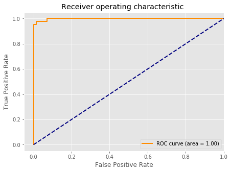
# 绘制ROC曲线：
from sklearn.metrics import roc_curve,auc
from sklearn.metrics import make_scorer,f1_score

scorer = make_scorer(f1_score,pos_label=0)
gs = GridSearchCV(estimator=pipe_svc,param_grid=param_grid,scoring=scorer,cv=10)
y_pred = gs.fit(X_train,y_train).decision_function(X_test)
#y_pred = gs.predict(X_test)
fpr,tpr,threshold = roc_curve(y_test, y_pred) 					# 计算真阳率和假阳率
roc_auc = auc(fpr,tpr) 											# 计算auc的值
plt.figure()
lw = 2
plt.figure(figsize=(7,5))
plt.plot(fpr, tpr, color='darkorange',
         lw=lw, label='ROC curve (area = %0.2f)' % roc_auc) 	# 假阳率为横坐标，真阳率为纵坐标做曲线
plt.plot([0, 1], [0, 1], color='navy', lw=lw, linestyle='--')
plt.xlim([-0.05, 1.0])
plt.ylim([-0.05, 1.05])
plt.xlabel('False Positive Rate')
plt.ylabel('True Positive Rate')
plt.title('Receiver operating characteristic ')
plt.legend(loc="lower right")
plt.show()

练习：施工中