


文章目录
Random Variable
c
d
f
:
‾
\underline{cdf:}
cdf:cumulative distribution function
F
(
x
)
=
P
(
X
≤
x
)
F(x)=P(X \leq x)
F(x)=P(X≤x)
p
m
f
:
‾
\underline{pmf:}
pmf:probability mass function(for discrete probability distribution )
(1)
p
(
x
)
≥
0
,
x
∈
X
p(x) \geq0,x \in X
p(x)≥0,x∈X
(2)
∑
x
∈
X
P
(
x
)
=
1
\sum\limits_{x \in X}P(x)=1
x∈X∑P(x)=1
p
d
f
:
‾
\underline{pdf:}
pdf:probability density function(for continuous probability distribution )
(1)
f
(
x
)
≥
0
f(x) \geq 0
f(x)≥0for all x,
(2)
∫
−
∞
∞
f
(
x
)
d
x
=
1
\int_{-\infty}^{\infty}f(x)dx=1
∫−∞∞f(x)dx=1
discrete distribution:
Poisson Distribution:
P
(
X
=
x
)
=
(
n
x
)
p
x
(
1
−
p
)
n
−
x
=
n
!
x
!
(
n
−
x
)
!
p
x
(
1
−
p
)
n
−
x
=
n
(
n
−
1
)
…
(
n
−
x
+
2
)
(
n
−
x
+
1
)
p
x
x
!
(
1
−
p
)
n
−
x
P(X = x)=\begin{pmatrix} n \\ x \end{pmatrix}p^{x}(1-p)^{n-x}=\frac{n!}{x!(n-x)!}p^{x}(1-p)^{n-x}=\\ \frac{n(n-1)\dots(n-x+2)(n-x+1)p^{x}}{x!}(1-p)^{n-x}
P(X=x)=(nx)px(1−p)n−x=x!(n−x)!n!px(1−p)n−x=x!n(n−1)…(n−x+2)(n−x+1)px(1−p)n−x
Let:
p
→
0
,
n
→
∞
p\rightarrow 0 ,n \rightarrow \infty
p→0,n→∞
P
(
λ
)
P(\lambda)
P(λ)
P
k
=
λ
k
k
!
e
−
λ
k
=
0
,
1
,
…
P_{k}=\frac{\lambda^{k}}{k!}e^{-\lambda}\quad k=0,1,\dots
Pk=k!λke−λk=0,1,…
Negative Binomial Distribution
(
k
+
r
−
1
k
)
=
(
k
+
r
−
1
)
!
k
!
(
r
−
1
)
!
=
(
k
+
r
−
1
)
(
k
+
r
−
2
)
…
(
r
)
k
!
=
(
−
1
)
k
(
−
k
−
r
+
1
)
(
−
k
−
r
+
2
)
…
(
−
r
)
k
!
=
(
−
1
)
k
(
−
r
k
)
\left(\begin{array}{c}{k+r-1} \\ {k}\end{array}\right)=\frac{(k+r-1) !}{k !(r-1) !}=\frac{(k+r-1)(k+r-2) \ldots(r)}{k !}=(-1)^{k} \frac{(-k-r+1)(-k-r+2) \ldots(-r)}{k !}=(-1)^{k}\left(\begin{array}{c}{-r} \\ {k}\end{array}\right)
(k+r−1k)=k!(r−1)!(k+r−1)!=k!(k+r−1)(k+r−2)…(r)=(−1)kk!(−k−r+1)(−k−r+2)…(−r)=(−1)k(−rk)
continuous distribution:
Normal distibution:KaTeX parse error: Expected group after '_' at position 5: \int_̲\limits{\mathbb…
∫
0
∞
exp
(
−
x
2
2
)
d
x
=
1
2
\int_{0}^{\infty}\exp \left(-\frac{x^{2}}{2}\right) \mathrm{d} x=\frac{1}{2}
∫0∞exp(−2x2)dx=21
X
↬
N
(
μ
,
σ
2
)
X \looparrowright N(\mu,\sigma^2)
X↬N(μ,σ2)
pdf:
p
(
x
)
=
1
2
π
σ
e
−
(
x
−
μ
)
2
2
σ
2
p(x)=\frac{1}{\sqrt{2\pi}\sigma}e^{\frac{-(x-\mu)^2}{2\sigma^2}}
p(x)=2πσ1e2σ2−(x−μ)2
cdf:
F
(
x
)
=
1
2
π
σ
∫
−
∞
x
e
−
(
t
−
μ
)
2
2
σ
2
d
t
F(x)=\frac{1}{\sqrt{2\pi}\sigma}\int_{-\infty}^xe^{\frac{-(t-\mu)^2}{2\sigma^2}}dt
F(x)=2πσ1∫−∞xe2σ2−(t−μ)2dt
条件期望与重期望
条件期望的定义:
E ( x ∣ y ) = ∫ − ∞ ∞ x f ( x ∣ y ) d x E(x|y)=\int_{-\infty}^{\infty}xf(x|y)dx E(x∣y)=∫−∞∞xf(x∣y)dx(连续)
E ( x ∣ y ) = ∑ i x i ρ ( X = x i ∣ Y = y i ) E(x|y)=\sum\limits_ix_i\rho(X=x_i|Y=y_i) E(x∣y)=i∑xiρ(X=xi∣Y=yi)(离散)
重期望的性质
1. E ( E ( g ( x ) ∣ Y ) ) = ∫ − ∞ ∞ E ( E ( g ( x ) ∣ Y ) ) f Y ( y ) d y 1.E(E(g(x)|Y))=\int_{-\infty}^{\infty}E(E(g(x)|Y))f_{Y}(y)dy 1.E(E(g(x)∣Y))=∫−∞∞E(E(g(x)∣Y))fY(y)dy
= ∫ − ∞ ∞ [ ∫ − ∞ ∞ g ( x ) f ( x ∣ y ) d x ] f Y ( y ) d y \int_{-\infty}^{\infty}[\int_{-\infty}^{\infty}g(x)f(x|y)dx]f_{Y}(y)dy ∫−∞∞[∫−∞∞g(x)f(x∣y)dx]fY(y)dy
= ∫ − ∞ ∞ ∫ − ∞ ∞ g ( x ) f ( x ∣ y ) f Y ( y ) d x d y \int_{-\infty}^{\infty}\int_{-\infty}^{\infty}g(x)f(x|y)f_{Y}(y)dxdy ∫−∞∞∫−∞∞g(x)f(x∣y)fY(y)dxdy
= ∫ − ∞ ∞ ∫ − ∞ ∞ g ( x ) f ( x ∣ y ) d x d y \int_{-\infty}^{\infty}\int_{-\infty}^{\infty}g(x)f(x|y)dxdy ∫−∞∞∫−∞∞g(x)f(x∣y)dxdy
= E ( g ( x ) ) E(g(x)) E(g(x))
多维随机变量及其联合分布
二维随机变量
若 X , Y X, Y X,Y是两个定义在同一个样本空间上的随机变量,则称 ( X , Y ) (X, Y) (X,Y)是二维随机变量
F
(
x
,
y
)
=
P
{
(
X
≤
x
)
∩
(
Y
≤
y
)
}
\boldsymbol{F}(\boldsymbol{x}, \boldsymbol{y})=\boldsymbol{P}\{(\boldsymbol{X} \leq \boldsymbol{x}) \cap(\boldsymbol{Y} \leq \boldsymbol{y})\}
F(x,y)=P{(X≤x)∩(Y≤y)}
这其实是一个很需要仔细想想的概念,我们从一个变量的分布函数,一个不等式关系来到一个多变量的随机变量的关系,
F
(
x
,
y
)
=
P
{
X
≤
x
,
Y
≤
y
}
\boldsymbol{F}(\boldsymbol{x}, \boldsymbol{y})=\boldsymbol{P}\{\boldsymbol{X} \leq \boldsymbol{x},\boldsymbol{Y} \leq \boldsymbol{y}\}
F(x,y)=P{X≤x,Y≤y}
这个是总的概念,我们来想想离散的随机变量和连续的随机变量在表达上会不会有区别
(
x
1
,
…
,
x
n
)
(x_1,\dots,x_n)
(x1,…,xn)为n维随机变量,
(
x
1
,
…
,
x
n
)
(x_1,\dots,x_n)
(x1,…,xn)的函数
Y
=
g
(
x
1
,
…
,
x
n
)
Y=g(x_1,\dots,x_n)
Y=g(x1,…,xn)为一维随机变量,由
(
x
1
,
…
,
x
n
)
(x_1,\dots,x_n)
(x1,…,xn)的联合分布,我们得出
Y
=
g
(
x
1
,
…
,
x
n
)
Y=g(x_1,\dots,x_n)
Y=g(x1,…,xn)
多维度离散随机变量
我们考虑泊松分布
X
↬
P
(
λ
)
X\looparrowright P(\lambda)
X↬P(λ)
Z
=
X
+
Y
Z=X+Y
Z=X+Y
P
(
λ
)
:
p
k
=
λ
k
k
!
e
−
λ
,
k
=
0
,
1
,
2
,
3
…
P(\lambda):p_k=\frac{\lambda^k}{k!}e^{-\lambda},k=0,1,2,3\dots
P(λ):pk=k!λke−λ,k=0,1,2,3…
(我们注意
Z
=
X
+
Y
Z=X+Y
Z=X+Y)
大数定律
定义:设 X n X_{n} Xn是一个随机变量序列, X X X为一个随机变量,如果对于任意的 ε > 0 \varepsilon > 0 ε>0,有 l i m n → ∞ P { ∣ X n − X ∣ ≥ ε } = 0 lim_{n \rightarrow \infty}P\{|X_n -X| \geq \varepsilon \}=0 limn→∞P{∣Xn−X∣≥ε}=0
称随机变量序列 X n {X_n} Xn依概率收敛于随机变量X
以上的例子说明一般按分布收敛与依概率收敛是不等价的.而下面的定理则说明:当极限随机变量为常数时,按分布收敛与依概率收敛是等价的.
X
n
⟶
P
X
⇒
X
n
⟶
L
X
X_{n} \stackrel{P}{\longrightarrow} X \Rightarrow X_{n} \stackrel{L}{\longrightarrow} X
Xn⟶PX⇒Xn⟶LX
X
n
⟶
P
a
⇔
X
n
⟶
L
a
X_{n} \stackrel{P}{\longrightarrow} a \Leftrightarrow X_{n} \stackrel{L}{\longrightarrow} a
Xn⟶Pa⇔Xn⟶La
统计量
现代统计学时期:
20世纪80年代开始,随着现代生物医学的发展,计算机技术的进步,人类对健康的管理和疾病的治疗已进入基因领域,对基因数据分析产生大量需求。多维海量的基因数据具有全新的数据特征,变量维度远远大于样本数,传统的统计方法失效了,因此一系列面向多维数据的统计分析方法相继产生,比如著名的Lasso方法。
20世纪90年代以来,随着Internet的发展,数据库中积累了海量的数据。如何从海量的数据中挖掘有用的信息就变得越来越重要了,数据挖掘也就应运而生了。与数据挖掘比较接近的名词是机器学习,。因为机器学习算法中涉及了很多的统计学理论,与统计学的关系密切,也被称为统计学习。
经验分布函数:
将所得数据
x
1
,
x
2
,
…
,
x
n
x_1,x_2,\dots,x_n
x1,x2,…,xn重新排列为顺序统计量
x
1
∗
≤
x
2
∗
≤
⋯
≤
x
n
∗
x_{1}^{*} \leq x_{2}^{*} \leq \cdots \leq x_{n}^{*}
x1∗≤x2∗≤⋯≤xn∗
F
n
∗
(
x
)
=
{
0
x
<
x
1
∗
k
/
n
x
k
∗
≤
x
<
x
k
+
1
∗
k
=
1
,
2
,
⋯
,
n
−
1
1
x
≥
x
n
∗
F_{n}^{*}(x)=\left\{\begin{array}{cc}{0} & {x<x_{1}^{*}} \\ {k / n} & {x_{k}^{*} \leq x<x_{k+1}^{*} \quad k=1,2, \cdots, n-1} \\ {1} & {x \geq x_{n}^{*}}\end{array}\right.
Fn∗(x)=⎩⎨⎧0k/n1x<x1∗xk∗≤x<xk+1∗k=1,2,⋯,n−1x≥xn∗
为总体
X
X
X的经验分布函数
例子:
从一批标准重量为克的罐头中,随 机抽取8听:
8,-4,6 ,7, -2, 1, 0, 1测的误差
求总体
X
X
X的经验分布函数
F
n
(
x
)
=
{
0
x
<
−
7
1
/
8
−
7
≤
x
<
−
4
2
/
8
−
4
≤
x
<
−
2
3
/
8
−
2
≤
x
<
0
4
/
8
0
≤
x
<
1
6
/
8
1
≤
x
<
6
7
/
8
6
≤
x
<
8
1
x
≥
8
F_{n}(x)=\left\{\begin{array}{cc}{0} & {x<-7} \\ {1 / 8} & {-7 \leq x<-4} \\ {2 / 8} & {-4 \leq x<-2} \\ {3 / 8} & {-2 \leq x<0} \\ {4 / 8} & {0 \leq x<1} \\ {6 / 8} & {1 \leq x<6} \\ {7 / 8} & {6 \leq x<8} \\ {1} & {x \geq 8}\end{array}\right.
Fn(x)=⎩⎪⎪⎪⎪⎪⎪⎪⎪⎪⎪⎨⎪⎪⎪⎪⎪⎪⎪⎪⎪⎪⎧01/82/83/84/86/87/81x<−7−7≤x<−4−4≤x<−2−2≤x<00≤x<11≤x<66≤x<8x≥8
统计量:依赖于样本的函数
样本均值:
X
ˉ
=
X
ˉ
n
=
1
n
∑
i
=
1
n
X
i
\bar{X}=\bar{X}_{n}=\frac{1}{n} \sum_{i=1}^{n} X_{i}
Xˉ=Xˉn=n1∑i=1nXi(总体样本)
(分组样本)样本均值的近似公式:
x
ˉ
=
x
1
f
1
+
…
x
k
f
k
n
(
n
=
∑
i
=
1
k
f
i
)
\bar{x}=\frac{x_1f_1+\dots x_kf_k}{n} (n=\sum_{i=1}^{k}f_i)
xˉ=nx1f1+…xkfk(n=∑i=1kfi)
f
i
f_i
fi为第i组的频数,k为组数
样本k阶原点矩:
X
k
=
1
n
∑
i
=
1
n
X
i
k
X^{k}=\frac{1}{n} \sum_{i=1}^{n} X_{i}^{k}
Xk=n1∑i=1nXik
单个正态总体分布下的样本均值分布: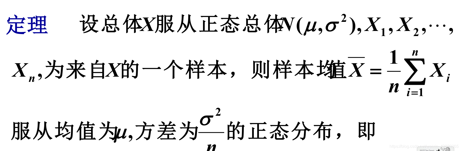
X
‾
=
1
n
∑
i
=
1
n
X
i
∼
N
(
μ
,
σ
2
n
)
\overline{\boldsymbol{X}}=\frac{1}{n} \sum_{i=1}^{n} X_{i} \sim N\left(\mu, \frac{\sigma^{2}}{n}\right)
X=n1∑i=1nXi∼N(μ,nσ2)
证明:
X
1
,
X
2
,
⋯
,
X
n
X_{1}, X_{2}, \cdots, X_{n}
X1,X2,⋯,Xn独立同分布,
E
(
X
i
)
=
μ
E(X_i)=\mu
E(Xi)=μ


Survey sampling
∙
\bullet
∙What is survey sampling?(c.f.census survey)(c.f.:参考,查看,来源于拉丁语)
∙
\bullet
∙understanding the whole by a
f
r
a
c
t
i
o
n
‾
\underline{fraction}
fraction(i.e.a
s
a
m
p
l
e
‾
\underline{sample}
sample)
Population:
Q:What is the population to survey?(In some cases,it can be difficult to identify or determine)
N:population size
a sample of size n:a subgroup of n members(n<N)
Q:Which n members should be included in the sample?(i.e.how to produce a
r
e
p
r
e
s
e
n
t
a
t
i
v
e
‾
\underline{representative}
representative sample)
quantity of interest:
x
i
,
i
=
1
,
2
,
3
⋯
N
x_i,i=1,2,3\cdots N
xi,i=1,2,3⋯N(each labeled by an integer)
x
i
x_i
xican be
n
u
m
e
r
i
c
a
l
‾
\underline{numerical}
numerical or
c
a
t
e
g
o
r
i
a
l
‾
\underline{categorial}
categorial
Multivariate
(
x
i
1
,
x
i
2
⋯
x
i
k
)
,
i
=
1
,
2
,
3
…
N
(x_{i1},x_{i2}\cdots x_{ik}),i=1,2,3 \dots N
(xi1,xi2⋯xik),i=1,2,3…N
D
e
f
i
n
i
t
i
o
n
:
‾
\underline{Definition : }
Definition:(survey sampling)
A technique to obtain
i
n
f
o
r
m
a
t
i
o
n
‾
\underline{information}
information about a
l
a
r
g
e
‾
\underline{large}
large population by examining only


 3264
3264


 被折叠的 条评论
为什么被折叠?
被折叠的 条评论
为什么被折叠?
 到【灌水乐园】发言


