


一、准备知识
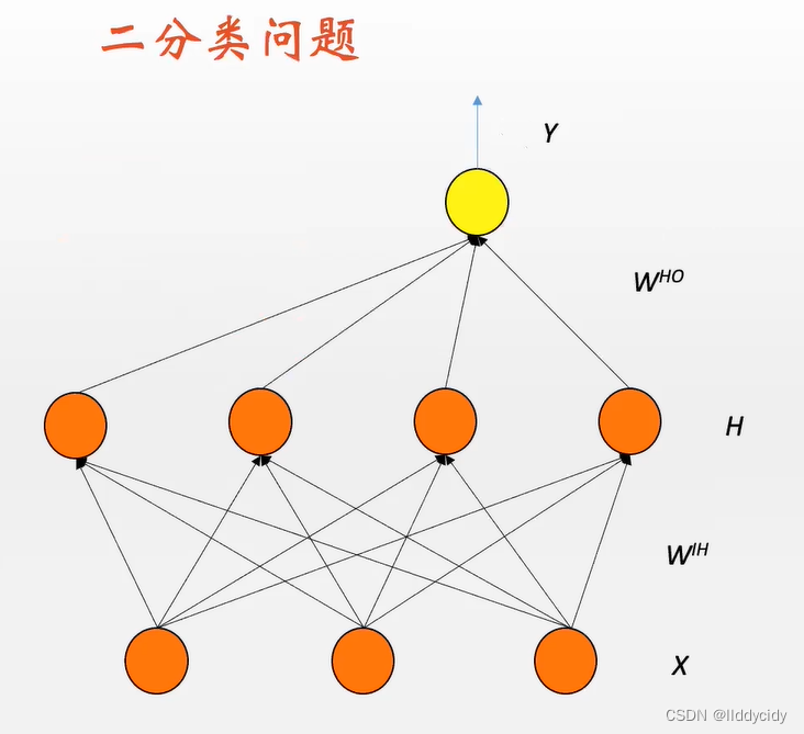
1.1看一个简单的二分类问题
Y
=
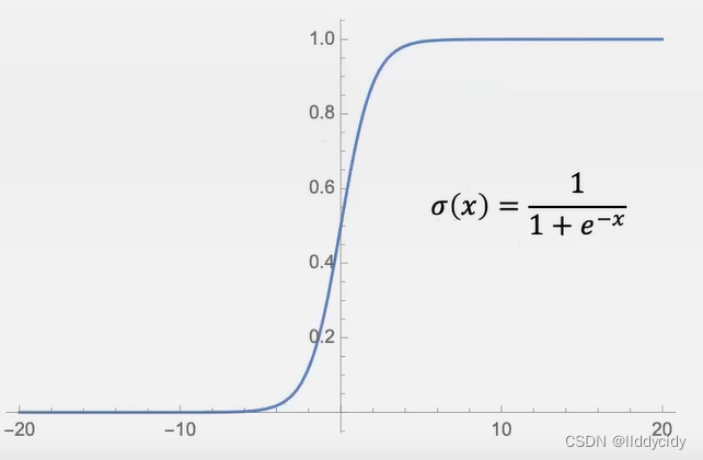
σ
(
σ
(
X
⋅
W
I
H
)
⋅
W
H
O
)
Out=1. if
Y
>
1
/
2
Out
=
0
. if
Y
<
1
/
2
\begin{array}{l} Y=\sigma\left(\sigma\left(X \cdot W^{I H}\right) \cdot W^{H O}\right) \\ \text { Out=1. if } Y>1 / 2 \\ \text { Out }=0 \text {. if } Y<1 / 2 \end{array}
Y=σ(σ(X⋅WIH)⋅WHO) Out=1. if Y>1/2 Out =0. if Y<1/2
观测神经网络的输出是否大于1/2
如何训练神经网络呢?本质就是调他的权重
那么我们
定义一个MSE目标函数,然后对他进行梯度下降,进而求他的权重
L
=
1
N
∑
i
=
1
N
(
Y
(
X
i
)
−
Z
i
)
2
L = \frac{1}{N} \sum_{i = 1}^{N}\left(Y\left(X_{i}\right)-Z_{i}\right)^{2}
L=N1i=1∑N(Y(Xi)−Zi)2
弊端:
并不是一个凸函数
在优化地形来看,
m
s
e
mse
mse目标函数就出现很多的局部最小点,对于优化问题的求解十分不利;
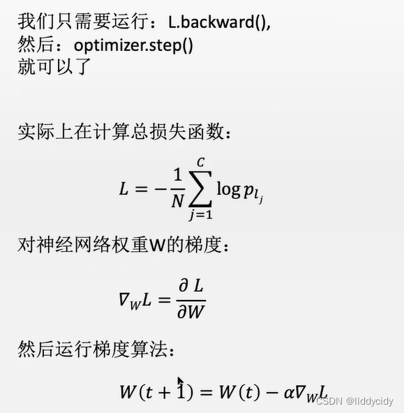
1.1.1换取另一种策略(交叉熵函数):
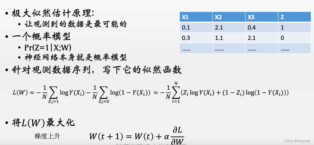
以下为公式详解:
简博士:极大似然估计
交叉熵函数公式详解
L
=
−
1
N
∑
i
=
1
N
Z
i
log
Y
(
X
i
)
+
(
1
−
Z
i
)
log
(
1
−
Y
(
X
i
)
)
L=-\frac{1}{N} \sum_{i=1}^{N} Z_{i} \log Y\left(X_{i}\right)+\left(1-Z_{i}\right) \log \left(1-Y\left(X_{i}\right)\right)
L=−N1i=1∑NZilogY(Xi)+(1−Zi)log(1−Y(Xi))
N
N
N项累加,第一部分为样本为1的分值,第二部分为样本为0的分值
例:当
Z
i
Z_{i}
Zi取1时,
(
1
−
Z
i
)
log
(
1
−
Y
(
X
i
)
\left(1-Z_{i}\right) \log \left(1-Y\left(X_{i}\right)\right.
(1−Zi)log(1−Y(Xi)项为0;同理
Z
i
Z_{i}
Zi为0 时,只有第二项
在得到梯度下降训练后的权重之后,就能对神经网络进行训练。
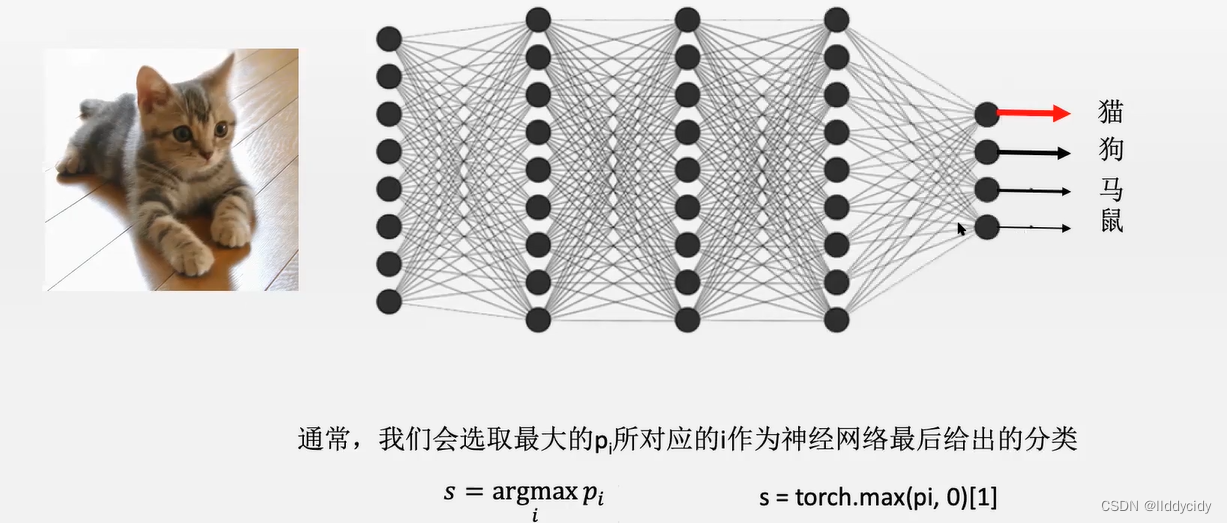
1.1.2准确率的计算(评估训练好的神经网络的质量)
一般评价分类器在测试数据中的好坏是用准确率计算,而不是交叉熵;(在测试集上计算)
(1)准确率(本质是对分类样本和测试集样本进行匹配)
r
=
N
right
N
=
#
(
argmax
i
p
i
=
C
i
)
N
Error
=
1
−
r
\begin{array}{l} r=\frac{N_{\text {right }}}{N}=\frac{\#\left(\operatorname{argmax}_{i} p_{i}=C_{i}\right)}{N}\\ \text { Error }=1-r \end{array}
r=NNright =N#(argmaxipi=Ci) Error =1−r
正确的样本除以样本总数
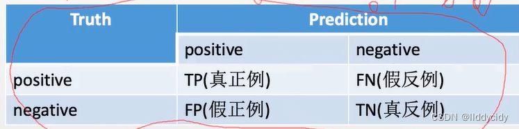
(2)confusion matrix
R
=
T
P
R
=
T
P
T
P
+
F
N
Recall
(
查全率)
True positive rate真正例率
F
P
R
=
F
P
T
N
+
F
P
False positive rate假正例率
\begin{array}{l} R=T P R=\frac{T P}{T P+F N} \quad \begin{array}{l} \text { Recall }(\text { 查全率) } \\ \text { True positive rate真正例率 } \end{array} \\ F P R=\frac{F P}{T N+F P} \quad \text { False positive rate假正例率 } \\ \end{array}
R=TPR=TP+FNTP Recall ( 查全率) True positive rate真正例率 FPR=TN+FPFP False positive rate假正例率
P
=
T
P
T
P
+
F
P
?
=
T
N
F
N
+
T
N
P=\frac{T P}{T P+F P} \quad ?=\frac{T N}{F N+T N}
P=TP+FPTP?=FN+TNTN
P
r
e
c
i
s
i
o
n
(查准率)
Precision(查准率)
Precision(查准率)
A
c
c
u
r
a
c
y
:
a
c
c
=
T
P
+
T
N
T
P
+
T
N
+
F
N
+
F
P
Accuracy: \quad a c c=\frac{T P+T N}{T P+T N+F N+F P}
Accuracy:acc=TP+TN+FN+FPTP+TN
(3)参数的选择
当判定界限不一样的时候,判定的结果也会不同
Y
=
σ
(
σ
(
X
⋅
W
I
H
)
⋅
W
H
O
)
Out=1. if
Y
>
θ
Out=0. if
Y
<
θ
\begin{array}{r} Y=\sigma\left(\sigma\left(X \cdot W^{I H}\right) \cdot W^{H O}\right) \\ \text { Out=1. if } Y>\theta \\ \text { Out=0. if } Y<\theta \end{array}
Y=σ(σ(X⋅WIH)⋅WHO) Out=1. if Y>θ Out=0. if Y<θ
横坐标:FPR:假正利率
纵坐标:TPR:真正例率

让
θ
⟶
[
0
,
1
]
\theta \longrightarrow [0,1]
θ⟶[0,1]
在0~1内进行取值


A
U
C
AUC
AUC就是求面积的和 类似于求积分
随机相当于是0.5概率(瞎猜)
1.2神经网络的多分类(交叉熵)
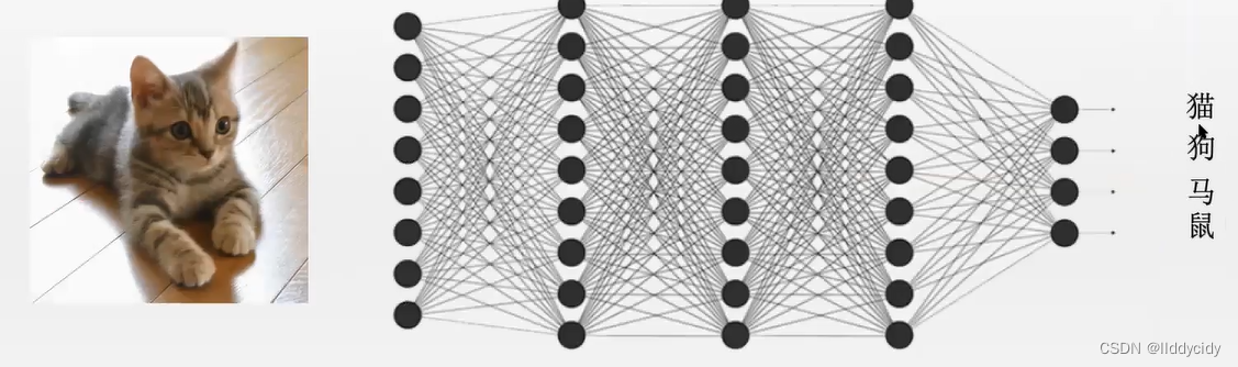
通常情况下:输入
N
N
N多少输出
N
N
N就是多少
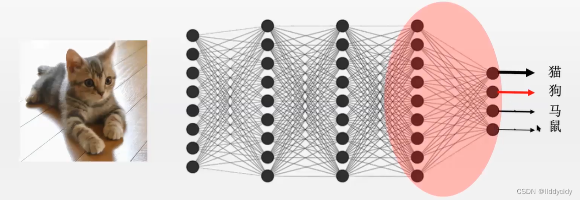
每个神经元的输出有不同的强度
p
i
p_{i}
pi,并且满足
∑
i
N
p
i
=
1
\sum_{i}^{N} p_{i}=1
∑iNpi=1
都是独立的,仅用前馈的话,并不能保证输出的范围在
[
0
,
1
]
[0,1]
[0,1]区间内,这时需要进行
s
o
f
t
m
a
x
softmax
softmax
p
i
=
softmax
(
y
i
=
∑
j
=
1
M
w
j
i
x
j
)
,
softmax
(
y
i
)
=
exp
(
y
i
)
∑
i
exp
(
y
i
)
nn.softmax(yi)
p_{i}=\operatorname{softmax}\left(y_{i}=\sum_{j=1}^{M} w_{j i} x_{j}\right), \operatorname{softmax}\left(y_{i}\right)=\frac{\exp \left(y_{i}\right)}{\sum_{i} \exp \left(y_{i}\right)} \quad \text { nn.softmax(yi) }
pi=softmax(yi=j=1∑Mwjixj),softmax(yi)=∑iexp(yi)exp(yi) nn.softmax(yi)

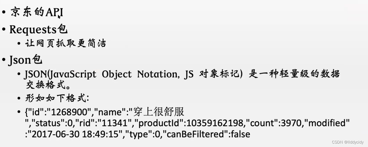
二、文本分类

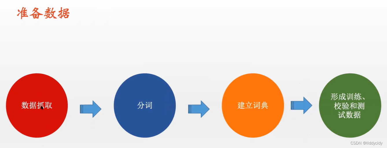
数据集准备:
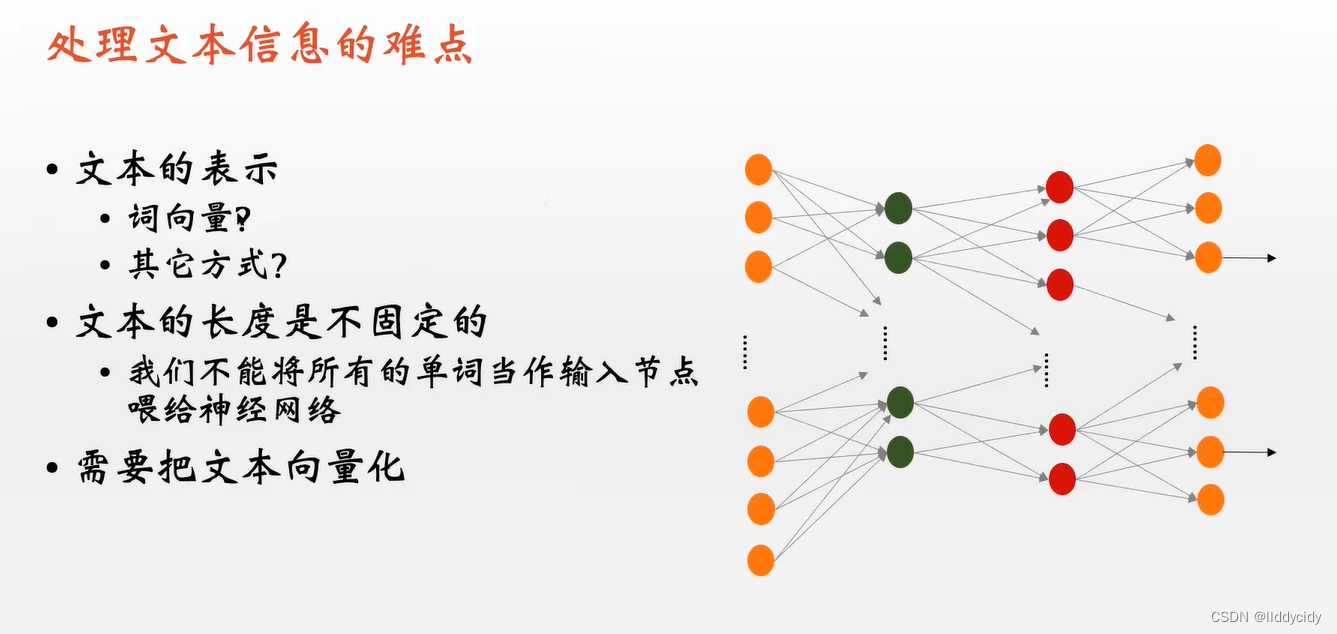
步骤:
注:vetor dim = len(words)
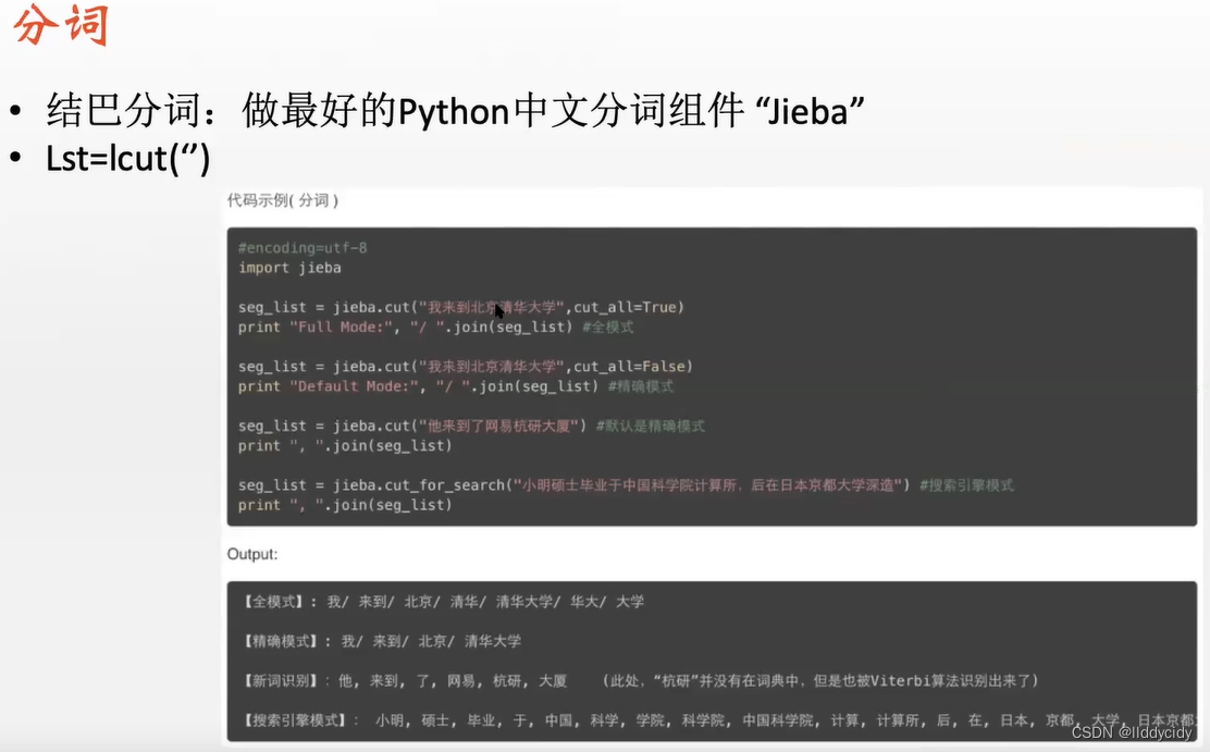
pip install jieba
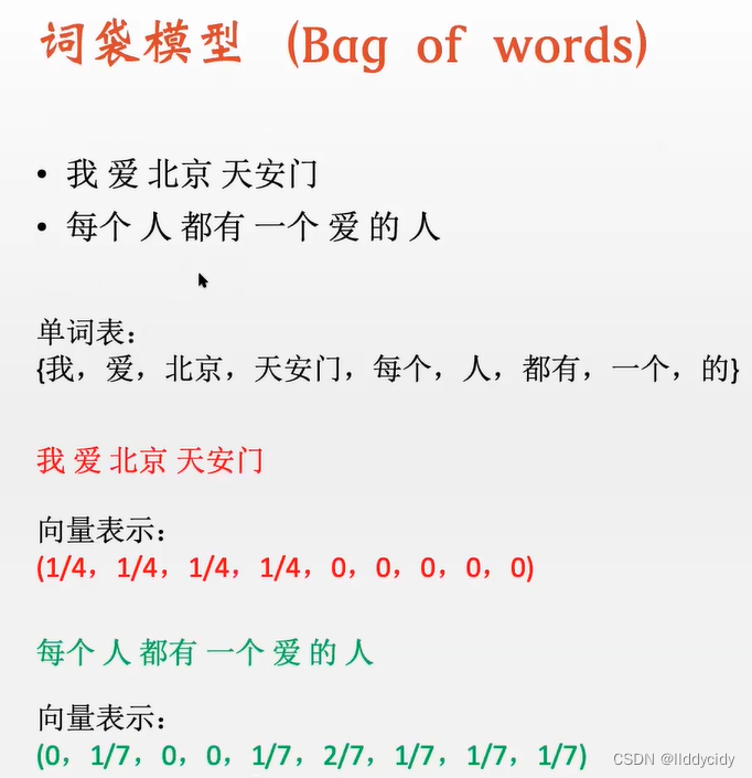
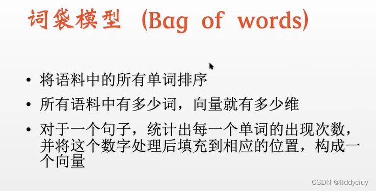
我 爱 北京 天安门 一共为4个word

因此总数为4 len(句子)
列表表示为

“我”在列表出现,因此加1(不是一一对应的 只要出现就加一)
1/4 = 我
向量表示:


注:词袋模型不能区分语义顺序;
例如:
我爱你 = 你爱我


源码:
代码
参考
1、LESSON 10.1&10.2&10.3 SSE与二分类交叉熵损失函数&二分类交叉熵损失函数的pytorch实现&多分类交叉熵损失函数
2、[Pytorch]交叉熵损失函数 CrossEntropyLoss() 详解
3、 [TensorFlow] 交叉熵损失函数,加权交叉熵损失函数
4、最全的交叉熵损失函数(Pytorch)
5、简博士—【合集】十分钟 机器学习 系列视频 《统计学习方法》


 780
780


 被折叠的 条评论
为什么被折叠?
被折叠的 条评论
为什么被折叠?
 到【灌水乐园】发言


