自然语言处理(NLP)编程实战-1.1 使用逻辑回归实现情感分类

内容汇总：https://blog.csdn.net/weixin_43093481/article/details/114989382?spm=1001.2014.3001.5501
课程笔记：1.1 监督学习与情感分析(Supervised ML & Sentiment Analysis)
代码：https://github.com/Ogmx/Natural-Language-Processing-Specialization
——————————————————————————————————————————

作业 1: 逻辑回归(Logistic Regression)

学习目标：
  学习逻辑回归，你将会学习使用逻辑回归对推特进行情感分析。给出一个推特，你要判断其是正向情感还是负向情感。

具体而言，将会学习：

• 给出一段文本，学习如何提取特征用于逻辑回归
• 从零开始实现逻辑回归
• 应用逻辑回归进行NLP任务
• 测试逻辑回归算法
• 进行错误分析

我们将使用一系列推特数据。在最后你的模型应该能得到99%的准确率。

导入函数和数据

# run this cell to import nltk
import nltk
from os import getcwd

下载数据

从该地址下载本实验需要的数据documentation for the twitter_samples dataset.

• twitter_samples: 执行以下命令来下载数据

nltk.download('twitter_samples')

• stopwords: 执行以下命令来下载停用词词典:

nltk.download('stopwords')

从 utils.py 导入帮助函数:

• process_tweet(): 清理文本、拆分单词、去停用词、词根化
• build_freqs(): 用于统计语料库中各单词被标记为"1"或"0"次数(即正向和负向情感)。然后构建"freqs"词典，其中键为(word,label) tuple，值为出现次数

# add folder, tmp2, from our local workspace containing pre-downloaded corpora files to nltk's data path
# this enables importing of these files without downloading it again when we refresh our workspace

filePath = f"{getcwd()}/../tmp2/"
nltk.data.path.append(filePath)

import numpy as np
import pandas as pd
from nltk.corpus import twitter_samples 

from utils import process_tweet, build_freqs

准备数据

• twitter_samples 中包含5000条正向推特数据集，5000条负向推特数据集，整体10,000条推特数据集
  • 如果直接使用3个数据集，将会包含重复推特
  • 因此只使用正向数据集和负向数据集

# select the set of positive and negative tweets
all_positive_tweets = twitter_samples.strings('positive_tweets.json')
all_negative_tweets = twitter_samples.strings('negative_tweets.json')

• 数据划分: 20% 作为测试集, 80% 作为训练集

# split the data into two pieces, one for training and one for testing (validation set) 
test_pos = all_positive_tweets[4000:]
train_pos = all_positive_tweets[:4000]
test_neg = all_negative_tweets[4000:]
train_neg = all_negative_tweets[:4000]

train_x = train_pos + train_neg 
test_x = test_pos + test_neg

• 对正向标签和负向标签建立numpy数组

# combine positive and negative labels
train_y = np.append(np.ones((len(train_pos), 1)), np.zeros((len(train_neg), 1)), axis=0)
test_y = np.append(np.ones((len(test_pos), 1)), np.zeros((len(test_neg), 1)), axis=0)

# Print the shape train and test sets
print("train_y.shape = " + str(train_y.shape))
print("test_y.shape = " + str(test_y.shape))

train_y.shape = (8000, 1)
test_y.shape = (2000, 1)

• 使用 build_freqs() 函数构建频率词典.
  • 强烈建议在 utils.py 中阅读 build_freqs() 函数代码来理解其原理

    for y,tweet in zip(ys, tweets):
        for word in process_tweet(tweet):
            pair = (word, y)
            if pair in freqs:
                freqs[pair] += 1
            else:
                freqs[pair] = 1

# create frequency dictionary
freqs = build_freqs(train_x, train_y)

# check the output
print("type(freqs) = " + str(type(freqs)))
print("len(freqs) = " + str(len(freqs.keys())))

type(freqs) = <class ‘dict’>
len(freqs) = 11346

处理推特

使用 process_tweet() 函数对推特中的每个单词进行向量化，去停用词和词根化

# test the function below
print('This is an example of a positive tweet: \n', train_x[0])
print('\nThis is an example of the processed version of the tweet: \n', process_tweet(train_x[0]))

This is an example of a positive tweet:
#FollowFriday @France_Inte @PKuchly57 @Milipol_Paris for being top engaged members in my community this week 😃
This is an example of the processed version of the tweet:
[‘followfriday’, ‘top’, ‘engag’, ‘member’, ‘commun’, ‘week’, ‘😃’]

Part 1: 逻辑回归

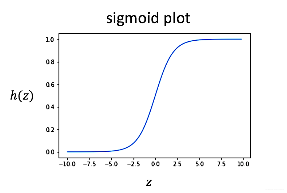
Part 1.1: Sigmoid

将会学习如何用逻辑回归进行文本分类

• sigmoid 函数定义：

$$h(z)=\frac{1}{1+{\exp }^{-z}}\text{\hspace{1em}(1)}$$
将输入’z’映射到0~1的区间中，也可以将其理解为概率

Hints

• numpy.exp

# UNQ_C1 (UNIQUE CELL IDENTIFIER, DO NOT EDIT)
def sigmoid(z): 
    '''
    Input:
        z: is the input (can be a scalar or an array)
    Output:
        h: the sigmoid of z
    '''
    
    ### START CODE HERE (REPLACE INSTANCES OF 'None' with your code) ###
    # calculate the sigmoid of z
    h = 1/(1+np.exp(-z))
    ### END CODE HERE ###
    
    return h

# Testing your function 
if (sigmoid(0) == 0.5):
    print('SUCCESS!')
else:
    print('Oops!')

if (sigmoid(4.92) == 0.9927537604041685):
    print('CORRECT!')
else:
    print('Oops again!')

SUCCESS!
CORRECT!

逻辑回归: 回归与sigmoid

逻辑回归采用一种标准线性回归方法，并用sigmoid函数作为激活函数

回归:
$$z={\theta }_0{x}_0+{\theta }_1{x}_1+{\theta }_2{x}_2+...{\theta }_N{x}_N$$
其中 $\theta$ 表示权值. 在深度学习中常用 w 向量表示. 在本实验中，用 $\theta$ 来表示权值

逻辑回归：
$$h(z)=\frac{1}{1+{\exp }^{-z}}$$
$$z={\theta }_0{x}_0+{\theta }_1{x}_1+{\theta }_2{x}_2+...{\theta }_N{x}_N$$
其中 ‘z’ 为’logits’，即输出.

Part 1.2 损失函数与梯度

使用全部样本的平均对数损失作为逻辑回归的损失函数：

$$J(\theta )=-\frac{1}{m}\sum _{i=1}^m{y}^{(i)}\log (h(z(\theta {)}^{(i)}))+(1-y^{(i)})\log (1-h(z(\theta {)}^{(i)}))\text{\hspace{1em}(5)}$$

• $m$ 是训练样本数
• $y^{(i)}$ 是第i个样本的真实标签
• $h(z(\theta {)}^{(i)})$ 是模型预测的第i个样本的标签

对一个训练样本的损失函数：
$$Loss=-1\times \left(y^{(i)}\log (h(z(\theta {)}^{(i)}))+(1-y^{(i)})\log (1-h(z(\theta {)}^{(i)}))\right)$$

• 所有$h$值为0~1,其对数为负，因此需要在最前面乘上-1
• 当模型预测结果为1 ($h(z(\theta ))=1$)， $y$ 的真实标签也为1时，则该样本损失值为0
• 同理，模型预测结果为0 ($h(z(\theta ))=0$)， $y$ 的真实标签也为0时，则该样本损失值为0
• 然而，当模型预测结果接近1 ($h(z(\theta ))=0.9999$)，真实标签为0时，第二项的对数损失将为一个很大的负数，当乘上-1后，变为很大的正数。$-1\times (1-0)\times log(1-0.9999)\approx 9.2$ 即预测值与真实值相差越大，损失值越大

# verify that when the model predicts close to 1, but the actual label is 0, the loss is a large positive value
-1 * (1 - 0) * np.log(1 - 0.9999) # loss is about 9.2

9.210340371976294

• 同理，如果模型预测结果接近0 ($h(z)=0.0001$)，而真实标签为1时，第一项的损失值很大： $-1\times log(0.0001)\approx 9.2$。

# verify that when the model predicts close to 0 but the actual label is 1, the loss is a large positive value
-1 * np.log(0.0001) # loss is about 9.2

9.210340371976182

更新权值

为了更新权值向量 $\theta$, 将使用梯度下降法来迭代提升模型表现
以${\theta }_j$为权值计算出的的损失函数$J$的梯度为：
$${\nabla }_{{\theta }_j}J(\theta )=\frac{1}{m}\sum _{i=1}^m(h^{(i)}-y^{(i)})x_j\text{\hspace{1em}(5)}$$

• ‘i’ 是全部’m’个训练样本的索引
• ‘j’ 是权值 ${\theta }_j$ 的索引, 而 $x_j$ 是与 ${\theta }_j$ 相匹配的特征
• 通过减去一部分梯度值来更新权值 ${\theta }_j$，该部分由学习率 $\alpha$ 决定
  $${\theta }_j={\theta }_j-\alpha \times {\nabla }_{{\theta }_j}J(\theta )$$
• 学习率 $\alpha$ 用来控制每步更新的大小/幅度

实现梯度下降

• 迭代次数 num_iters 是使用整个训练集的次数.
• 在每次迭代中，都要用全部训练样本计算损失函数(共m个训练样本)
• 不是一次更新一个权值 ${\theta }_i$，而是更新所有权值用向量表示为：
  $$\theta =\left(\begin{array}{c}{\theta }_0\\ {\theta }_1\\ {\theta }_2\\ ⋮\\ {\theta }_n\end{array}\right)$$
• $\theta$ 的维度为 (n+1, 1), 其中 ‘n’ 是特征数, 用 ${\theta }_0$ 表示偏差(bias) (与其相匹配的特征值 ${\mathbf{x}}_0$ 为 1).
• 输出 ‘logits’, ‘z’, 通过特征矩阵’x’与权值向量’theta’相乘得到 $z=\mathbf{x}\theta$
  • $\mathbf{x}$ 的维度为 (m, n+1)
  • $\theta$: 的维度为 (n+1, 1)
  • $\mathbf{z}$: 的维度为 (m, 1)
• 预测值 ‘h’, 通过对输出’z’应该sigmoid函数得到: $h(z)=sigmoid(z)$, 其维度为 (m,1).
• 损失函数 $J$ 通过对向量 ‘y’ 和 ‘log(h)’ 计算点乘得到，因为’y’ 和 ‘h’ 都是维度为 (m,1) 的列向量, 转置左侧的向量, 使用矩阵乘法即可计算各行和各列的点乘
  $$J=\frac{-1}{m}\times \left({\mathbf{y}}^T\cdot log(\mathbf{h})+{(1-\mathbf{y})}^T\cdot log(1-\mathbf{h})\right)$$
• 对于theta的更新同样是向量化的。因为 $\mathbf{x}$ 的维度为 (m, n+1), $\mathbf{h}$ 和 $\mathbf{y}$ 的维度都是 (m, 1), 需要对 $\mathbf{x}$ 进行转置然后将其放在左侧以进行矩阵乘法，最终得到的结果维度为 (n+1, 1) :
  $$\theta =\theta -\frac{\alpha }{m}\times \left({\mathbf{x}}^T\cdot \left(\mathbf{h}-\mathbf{y}\right)\right)$$

Hints

• 使用 np.dot 实现矩阵乘法.
• 确保 -1/m 为浮点数, 对分子或分母 (或全部), 使用 `float(1)`, 或 `1.` 将其转换为float类型.

# UNQ_C2 (UNIQUE CELL IDENTIFIER, DO NOT EDIT)
def gradientDescent(x, y, theta, alpha, num_iters):
    '''
    Input:
        x: matrix of features which is (m,n+1)
        y: corresponding labels of the input matrix x, dimensions (m,1)
        theta: weight vector of dimension (n+1,1)
        alpha: learning rate
        num_iters: number of iterations you want to train your model for
    Output:
        J: the final cost
        theta: your final weight vector
    Hint: you might want to print the cost to make sure that it is going down.
    '''
    ### START CODE HERE (REPLACE INSTANCES OF 'None' with your code) ###
    # get 'm', the number of rows in matrix x
    m = x.shape[0]
    
    for i in range(0, num_iters):
        
        # get z, the dot product of x and theta
        z = np.dot(x,theta)
        
        # get the sigmoid of z
        h = sigmoid(z)
        
        # calculate the cost function
        J = -1/m * (np.dot(y.T,np.log(h)) + np.dot((1-y).T,np.log(1-h)))

        # update the weights theta
        theta = theta - alpha/m * (np.dot(x.T,(h-y)))
        
    ### END CODE HERE ###
    J = float(J)
    return J, theta

# Check the function
# Construct a synthetic test case using numpy PRNG functions
np.random.seed(1)
# X input is 10 x 3 with ones for the bias terms
tmp_X = np.append(np.ones((10, 1)), np.random.rand(10, 2) * 2000, axis=1)
# Y Labels are 10 x 1
tmp_Y = (np.random.rand(10, 1) > 0.35).astype(float)

# Apply gradient descent
tmp_J, tmp_theta = gradientDescent(tmp_X, tmp_Y, np.zeros((3, 1)), 1e-8, 700)
print(f"The cost after training is {tmp_J:.8f}.")
print(f"The resulting vector of weights is {[round(t, 8) for t in np.squeeze(tmp_theta)]}")

The cost after training is 0.67094970.
The resulting vector of weights is [4.1e-07, 0.00035658, 7.309e-05]

Part 2: 提取特征

• 给出一系列推特，提取其特征并存入矩阵中，将提取两类特征
  • 第一类特征是该推特中正向词出现次数
  • 第二类特征是该推特中负向词出现次数
• 然后应用这些特征训练逻辑回归分类器.
• 在测试集上测试该模型

实现 extract_features 函数

• 该函数针对单个推特进行特征提取.
• 使用 process_tweet() 函数处理推特并用列表存储推特中单词.
• 使用循环依次处理列表中的各单词
  • 对于每个单词, 通过 freqs 字典，统计其被标记为’1’的次数 (即查找键 (word, 1.0)）
  • 同上，统计其被标记为’0’的次数. (即查找键 (word, 0.0))

Hints

• 处理好当 (word, label) 键不在字典中的情况.
• 关于 `.get()` 的用法. 例子 example

# UNQ_C3 (UNIQUE CELL IDENTIFIER, DO NOT EDIT)
def extract_features(tweet, freqs):
    '''
    Input: 
        tweet: a list of words for one tweet
        freqs: a dictionary corresponding to the frequencies of each tuple (word, label)
    Output: 
        x: a feature vector of dimension (1,3)
    '''
    # process_tweet tokenizes, stems, and removes stopwords
    word_l = process_tweet(tweet)
    
    # 3 elements in the form of a 1 x 3 vector
    x = np.zeros((1, 3)) 
    
    #bias term is set to 1
    x[0,0] = 1 
    
    ### START CODE HERE (REPLACE INSTANCES OF 'None' with your code) ###
    
    # loop through each word in the list of words
    for word in word_l:
        
        # increment the word count for the positive label 1
        x[0,1] += freqs.get((word,1),0)
        
        # increment the word count for the negative label 0
        x[0,2] += freqs.get((word,0),0)
        
    ### END CODE HERE ###
    assert(x.shape == (1, 3))
    return x

# Check your function

# test 1
# test on training data
tmp1 = extract_features(train_x[0], freqs)
print(tmp1)

[[1.00e+00 3.02e+03 6.10e+01]]

# test 2:
# check for when the words are not in the freqs dictionary
tmp2 = extract_features('blorb bleeeeb bloooob', freqs)
print(tmp2)

[[1. 0. 0.]]

Part 3: 训练模型

为了训练模型:

• 将各训练样本的特征构成矩阵 X.
• 使用之前实现的 gradientDescent 函数进行梯度下降

# collect the features 'x' and stack them into a matrix 'X'
X = np.zeros((len(train_x), 3))
for i in range(len(train_x)):
    X[i, :]= extract_features(train_x[i], freqs)

# training labels corresponding to X
Y = train_y

# Apply gradient descent
J, theta = gradientDescent(X, Y, np.zeros((3, 1)), 1e-9, 1500)
print(f"The cost after training is {J:.8f}.")
print(f"The resulting vector of weights is {[round(t, 8) for t in np.squeeze(theta)]}")

The cost after training is 0.24216529.
The resulting vector of weights is [7e-08, 0.0005239, -0.00055517]

Part 4: 测试逻辑回归模型

为了测试逻辑回归模型，应输入一些非样本数据，即模型从未见过的数据

实现函数： predict_tweet

预测一个推特是正向还是负向

• 给出一个推特，对其进行预处理和特征提取.
• 对提取出的特征应用训练好的模型得到输出’z’
• 对输出’z’使用sigmoid函数，得到最终预测结果 (一个0~1之间的值).
  $$y_{pred}=sigmoid(\mathbf{x}\cdot \theta )$$

# UNQ_C4 (UNIQUE CELL IDENTIFIER, DO NOT EDIT)
def predict_tweet(tweet, freqs, theta):
    '''
    Input: 
        tweet: a string
        freqs: a dictionary corresponding to the frequencies of each tuple (word, label)
        theta: (3,1) vector of weights
    Output: 
        y_pred: the probability of a tweet being positive or negative
    '''
    ### START CODE HERE (REPLACE INSTANCES OF 'None' with your code) ###
    
    # extract the features of the tweet and store it into x
    x = extract_features(tweet,freqs)
    
    # make the prediction using x and theta
    y_pred = sigmoid(np.dot(x,theta))
    
    ### END CODE HERE ###
    
    return y_pred

# Run this cell to test your function
for tweet in ['I am happy', 'I am bad', 'this movie should have been great.', 'great', 'great great', 'great great great', 'great great great great']:
    print( '%s -> %f' % (tweet, predict_tweet(tweet, freqs, theta)))

I am happy -> 0.518580
I am bad -> 0.494339
this movie should have been great. -> 0.515331
great -> 0.515464
great great -> 0.530898
great great great -> 0.546273
great great great great -> 0.561561

使用测试集测试模型效果

在使用训练集对模型进行训练后，使用测试集验证其在真实情况中的表现

实现函数 test_logistic_regression

• 给出测试数据和训练好的模型权值，计算模型预测准确率
• 使用predict_tweet()函数对测试集中每条推特进行预测
• 如果预测值>0.5，则将模型分类结果y_hat设为1，反之将y_hat设为0
• 当y_hat与test_y相等时，则认为预测准确。预测准确样本数除样本总数m，即为预测准确率

Hints

• 使用 np.asarray() 将 list 转换为numpy array
• 使用 np.squeeze() 将维度为 (m,1) 的array转化为维度为 (m,) 的array

# UNQ_C5 (UNIQUE CELL IDENTIFIER, DO NOT EDIT)
def test_logistic_regression(test_x, test_y, freqs, theta):
    """
    Input: 
        test_x: a list of tweets
        test_y: (m, 1) vector with the corresponding labels for the list of tweets
        freqs: a dictionary with the frequency of each pair (or tuple)
        theta: weight vector of dimension (3, 1)
    Output: 
        accuracy: (# of tweets classified correctly) / (total # of tweets)
    """
    
    ### START CODE HERE (REPLACE INSTANCES OF 'None' with your code) ###
    
    # the list for storing predictions
    y_hat = []
    
    for tweet in test_x:
        # get the label prediction for the tweet
        y_pred = predict_tweet(tweet, freqs, theta)
        
        if y_pred > 0.5:
            # append 1.0 to the list
            y_hat.append(1)
        else:
            # append 0 to the list
            y_hat.append(0)

    # With the above implementation, y_hat is a list, but test_y is (m,1) array
    # convert both to one-dimensional arrays in order to compare them using the '==' operator
    cnt=0
    test_y = test_y.squeeze()
    for i in range(0,len(y_hat)):
        if y_hat[i]==test_y[i]:
            cnt+=1
    accuracy = cnt / len(y_hat)

    ### END CODE HERE ###
    
    return accuracy

tmp_accuracy = test_logistic_regression(test_x, test_y, freqs, theta)
print(f"Logistic regression model's accuracy = {tmp_accuracy:.4f}")

Logistic regression model’s accuracy = 0.9950

Part 5: 错误分析

在该部分将会找出那些模型预测错误的推特，并分析为什么会出错？对于什么类型的推特会出错？

# Some error analysis done for you
print('Label Predicted Tweet')
for x,y in zip(test_x,test_y):
    y_hat = predict_tweet(x, freqs, theta)

    if np.abs(y - (y_hat > 0.5)) > 0:
        print('THE TWEET IS:', x)
        print('THE PROCESSED TWEET IS:', process_tweet(x))
        print('%d\t%0.8f\t%s' % (y, y_hat, ' '.join(process_tweet(x)).encode('ascii', 'ignore')))

Label Predicted Tweet
THE TWEET IS: @jaredNOTsubway @iluvmariah @Bravotv Then that truly is a LATERAL move! Now, we all know the Queen Bee is UPWARD BOUND : ) #MovingOnUp
THE PROCESSED TWEET IS: [‘truli’, ‘later’, ‘move’, ‘know’, ‘queen’, ‘bee’, ‘upward’, ‘bound’, ‘movingonup’]
1 0.49996890 b’truli later move know queen bee upward bound movingonup’
THE TWEET IS: @MarkBreech Not sure it would be good thing 4 my bottom daring 2 say 2 Miss B but Im gonna be so stubborn on mouth soaping ! #NotHavingit :p
THE PROCESSED TWEET IS: [‘sure’, ‘would’, ‘good’, ‘thing’, ‘4’, ‘bottom’, ‘dare’, ‘2’, ‘say’, ‘2’, ‘miss’, ‘b’, ‘im’, ‘gonna’, ‘stubborn’, ‘mouth’, ‘soap’, ‘nothavingit’, ‘:p’]
1 0.48622857 b’sure would good thing 4 bottom dare 2 say 2 miss b im gonna stubborn mouth soap nothavingit :p’
THE TWEET IS: I’m playing Brain Dots : ) #BrainDots
http://t.co/UGQzOx0huu
THE PROCESSED TWEET IS: [“i’m”, ‘play’, ‘brain’, ‘dot’, ‘braindot’]
1 0.48370665 b"i’m play brain dot braindot"
THE TWEET IS: I’m playing Brain Dots : ) #BrainDots http://t.co/aOKldo3GMj http://t.co/xWCM9qyRG5
THE PROCESSED TWEET IS: [“i’m”, ‘play’, ‘brain’, ‘dot’, ‘braindot’]
1 0.48370665 b"i’m play brain dot braindot"
THE TWEET IS: I’m playing Brain Dots : ) #BrainDots http://t.co/R2JBO8iNww http://t.co/ow5BBwdEMY
THE PROCESSED TWEET IS: [“i’m”, ‘play’, ‘brain’, ‘dot’, ‘braindot’]
1 0.48370665 b"i’m play brain dot braindot"
THE TWEET IS: off to the park to get some sunlight : )
THE PROCESSED TWEET IS: [‘park’, ‘get’, ‘sunlight’]
1 0.49578765 b’park get sunlight’
THE TWEET IS: @msarosh Uff Itna Miss karhy thy ap :p
THE PROCESSED TWEET IS: [‘uff’, ‘itna’, ‘miss’, ‘karhi’, ‘thi’, ‘ap’, ‘:p’]
1 0.48199810 b’uff itna miss karhi thi ap :p’
THE TWEET IS: @phenomyoutube u probs had more fun with david than me : (
THE PROCESSED TWEET IS: [‘u’, ‘prob’, ‘fun’, ‘david’]
0 0.50020353 b’u prob fun david’
THE TWEET IS: pats jay : (
THE PROCESSED TWEET IS: [‘pat’, ‘jay’]
0 0.50039294 b’pat jay’
THE TWEET IS: my beloved grandmother : ( https://t.co/wt4oXq5xCf
THE PROCESSED TWEET IS: [‘belov’, ‘grandmoth’]
0 0.50000002 b’belov grandmoth’

在后续课程中，将会学习如何用深度学习的方法来提升预测效果

Part 6: 预测你自己的推特

# Feel free to change the tweet below
my_tweet = 'This is a ridiculously bright movie. The plot was terrible and I was sad until the ending!'
print(process_tweet(my_tweet))
y_hat = predict_tweet(my_tweet, freqs, theta)
print(y_hat)
if y_hat > 0.5:
    print('Positive sentiment')
else: 
    print('Negative sentiment')

[‘ridicul’, ‘bright’, ‘movi’, ‘plot’, ‘terribl’, ‘sad’, ‘end’]
[[0.48139087]]
Negative sentiment