plot 二维、三维可视化

1.二维可视化

（1）相关代码

def show(X, label,ep):
    # t-SNE embedding of the digits dataset
    tsne = manifold.TSNE(n_components=2, init='pca', random_state=0)
    X_tsne = tsne.fit_transform(X)
    print("plot_embedding is start")
    plot_embedding(X_tsne, np.array(label))
    path = "./show_cosine/" + str(ep)  + "plt"
    plt.savefig(path)
    plt.show()
    print("SAVE")

def plot_embedding(X, y):
    x_min, x_max = np.min(X, 0), np.max(X, 0)
    X = (X - x_min) / (x_max - x_min)
    
    plt.figure()
    ax = plt.subplot(111)

#为每个点添加对应的标签以及颜色
    for i in range(X.shape[0]):
        plt.text(X[i, 0], X[i, 1], y[i],
                 fontdict={'weight': 'bold', 'size': 5},
                 color=plt.cm.Set1(y[i] % 20),
                 )
    plt.xticks([]), plt.yticks([])

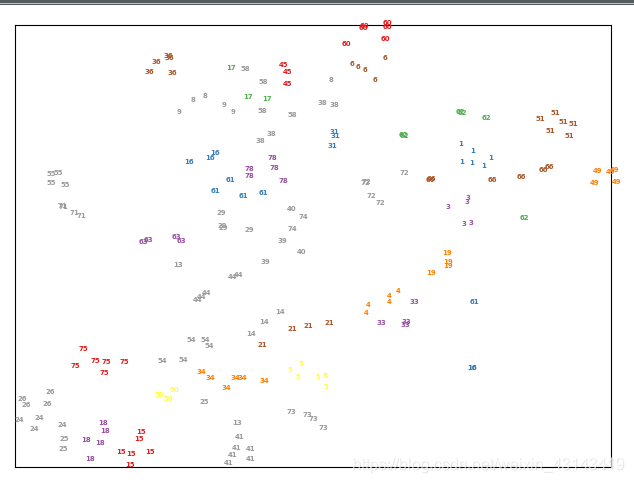
（2）可视化结果：

2.三维可视化

（1）相关代码

from sklearn import manifold  # true
import numpy as np
import pickle
import matplotlib.pyplot as plt  # true
from mpl_toolkits.mplot3d import Axes3D

def show(X, label,ep):
    # t-SNE embedding of the digits dataset
    tsne = manifold.TSNE(n_components=3, init='pca', random_state=0)
    X_tsne = tsne.fit_transform(X)
    print("plot_embedding is start")
    plot_embedding(X_tsne, np.array(label))
    path = "./test" + str(ep)  + "plt"
    plt.savefig(path)
    plt.draw()
    plt.pause(10)
    plt.close()
    print("SAVE")


def plot_embedding(X, y):
    x_min, x_max = np.min(X, 0), np.max(X, 0)
    X = (X - x_min) / (x_max - x_min)
    # plt.figure()
    #plt.subplot(111)
    ax=plt.subplot(projection='3d')
    for i in range(X.shape[0]):
        ax.scatter(X[i, 0], X[i, 1],X[i, 2], color=plt.cm.Set1(y[i]%15))

（2）可视化结果

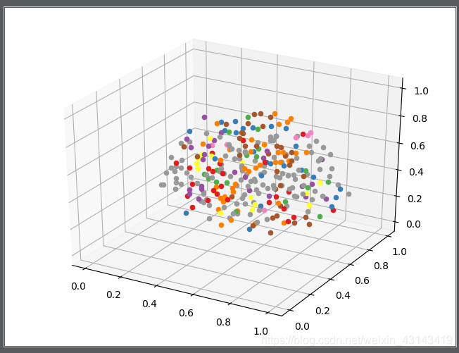
(3)三维可视化最好的工具是matlab
可进行角度的调整、转动，更有利于分析数据的分布特征