


 本文介绍了一种基于LSTM的船舶轨迹预测模型,通过单步和多步预测验证模型准确性,并展示了不同预测长度下的误差变化。
之前给的数据和代码可能有一些问题,现在从新修改一下,末尾提供数据集和源码链接
单步预测步长:10
单步循环预测长时间的位置:从第1个位置开始,前10个位置(真实位置)预测第11个位置,然后第2个位置到第11个位置(预测值)为一组,预测第12个位置,以此循环预测更长时间的值,其误差会随时间的延长而增加
多步预测:假设单步预测输入4个变量(lon,lat,cog,sog),则输出还是4个变量(lon,lat,cog,sog),若要直接预测两步的话,需要输出8个变量{下一时刻4个 + 下下一时刻4个},即(lon1, lat1, cog1, sog1, lon2, lat2, cog2, sog2)
1、工具包
import numpy as np
import tensorflow as tf
import pandas as pd
import matplotlib.pyplot as plt
from keras.layers.core import Dense, Activation, Dropout
from keras.layers import LSTM
from keras.models import Sequential, load_model
from keras.callbacks import CSVLogger, ReduceLROnPlateau
from keras.optimizers import adam_v2
import transbigdata as tbd
import warnings
warnings.filterwarnings("ignore")
# 设置种子参数,方便复现
np.random.seed(120)
tf.random.set_seed(120)
# 支持中文
plt.rcParams['font.sans-serif'] = ['SimHei']  # 用来正常显示中文标签
plt.rcParams['axes.unicode_minus'] = False  # 用来正常显示负号
2、读取数据
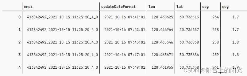
# 读取数据,updateDateFormat 为定位时间,两分钟一个点,mmsi 为轨迹 id
train = pd.read_csv("./train.csv",index_col=0)
test = pd.read_csv("./test.csv",index_col=0)
train.head()
3、提取特征和标签数据
每连续的 10 个位置为一组,预测下一个位置
def create_dataset(data, window=10,max_min):
    """
    :param data:  		轨迹数据集合
    :param window: 		多少个数据一组
    :param max_min:		用来归一化
    :return: 	  		数据、标签
    """
    train_seq = []
    train_label = []
    m, n = maxmin
    for traj_id in set(data['mmsi']):
        data_temp = data.loc[data.mmsi == traj_id]
        data_temp = np.array(data_temp.loc[:, ['lon', 'lat', 'sog', 'cog']])
        # 标准化
        data_temp = (data_temp - n) / (m - n)

        for i in range(data_temp.shape[0] - window):
            x = []
            for j in range(i, i + window):
                x.append(list(data_temp[j, :]))
            train_seq.append(x)
            train_label.append(data_temp[i + window, :])

    train_seq = np.array(train_seq, dtype='float64')
    train_label = np.array(train_label, dtype='float64')

    return train_seq, train_label
4、构建模型
def trainModel(train_X, train_Y, test_X, test_Y):
    model = Sequential()
    model.add(LSTM(108, input_shape=(train_X.shape[1], train_X.shape[2]), return_sequences=False))
    # model.add(Dropout(0.3))
    model.add(Dense(train_Y.shape[1]))
    model.add(Activation("relu"))
    adam = adam_v2.Adam(learning_rate=0.01)
    model.compile(loss='mse', optimizer=adam, metrics=['acc'])
    # 保存训练过程中损失函数和精确度的变化
    log = CSVLogger(f"./log.csv", separator=",", append=True)
    # 用来自动降低学习率
    reduce = ReduceLROnPlateau(monitor='val_acc', factor=0.5, patience=1, verbose=1,
                               mode='auto', min_delta=0.001, cooldown=0, min_lr=0.001)
	# 模型训练
    model.fit(train_X, train_Y, epochs=20, batch_size=32, verbose=1, validation_split=0.1,
                  callbacks=[log, reduce])
    # 用测试集评估
    loss, acc = model.evaluate(test_X, test_Y, verbose=1)
    print('Loss : {}, Accuracy: {}'.format(loss, acc * 100))
    # 保存模型
    model.save(f"./model.h5")
    # 打印神经网络结构,统计参数数目
    model.summary()
    return model
5、训练
# 计算归一化参数
nor = np.array(train.loc[:, ['lon', 'lat', 'sog', 'cog']])
m = nor.max(axis=0)
n = nor.min(axis=0)
maxmin = [m, n]
# 步长
windows = 10
# 训练集
train_seq, train_label= createSequence(train, windows, maxmin)
# 测试集
test_seq, test_label = createSequence(test, windows, maxmin)
# 训练模型,我只训练了20次,你可以训练 100 次,精度会更高
model = trainModel(train_seq, train_label,test_seq,test_label)
# 加载训练好的模型
# model = load_model("./model.h5")
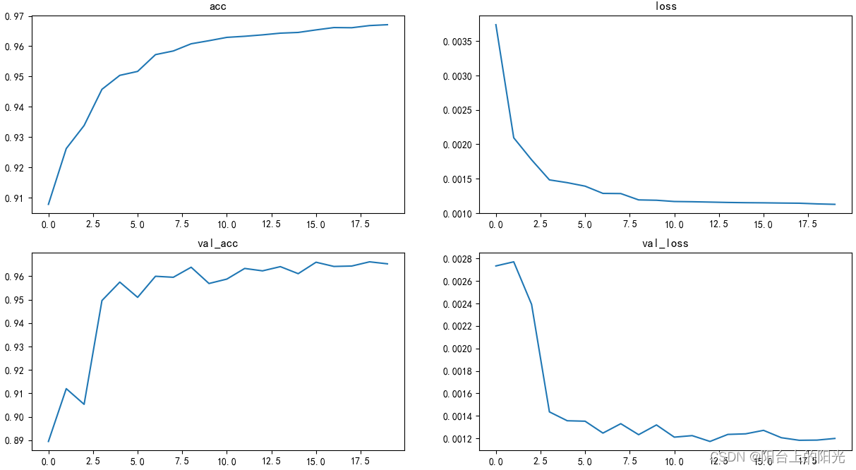
6、损失函数和准确率的变化
logs = pd.read_csv("./log.csv")

fig, ax = plt.subplots(2,2,figsize=(8,8))
ax[0][0].plot(logs['epoch'],logs['acc'], label='acc')
ax[0][0].set_title('acc')

ax[0][1].plot(logs['epoch'],logs['loss'], label='loss')
ax[0][1].set_title('loss')

ax[1][0].plot(logs['epoch'],logs['val_acc'], label='val_acc')
ax[1][0].set_title('val_acc')

ax[1][1].plot(logs['epoch'],logs['val_loss'], label='val_loss')
ax[1][1].set_title('val_loss')

plt.show()
7、预测
# 多维反归一化
def FNormalizeMult(y_pre, y_true, max_min):
    [m1, n1, s1, c1], [m2, n2, s2, c2] = max_min
    y_pre[:, 0] = y_pre[:, 0] * (m1 - m2) + m2
    y_pre[:, 1] = y_pre[:, 1] * (n1 - n2) + n2
    y_pre[:, 2] = y_pre[:, 2] * (s1 - s2) + s2
    y_pre[:, 3] = y_pre[:, 3] * (c1 - c2) + c2
    y_true[:, 0] = y_true[:, 0] * (m1 - m2) + m2
    y_true[:, 1] = y_true[:, 1] * (n1 - n2) + n2
    y_true[:, 2] = y_true[:, 2] * (s1 - s2) + s2
    y_true[:, 3] = y_true[:, 3] * (c1 - c2) + c2

    # 计算真实值和预测值偏差的距离
    y_pre = np.insert(y_pre, y_pre.shape[1],
                      get_distance_hav(y_true[:, 1], y_true[:, 0], y_pre[:, 1], y_pre[:, 0]), axis=1)

    return y_pre, y_true

def hav(theta):
    s = np.sin(theta / 2)
    return s * s
#  计算坐标在 WGS84 下的距离
def get_distance_hav(lat0, lng0, lat1, lng1):
    EARTH_RADIUS = 6371
    lat0 = np.radians(lat0)
    lat1 = np.radians(lat1)
    lng0 = np.radians(lng0)
    lng1 = np.radians(lng1)

    dlng = np.fabs(lng0 - lng1)
    dlat = np.fabs(lat0 - lat1)
    h = hav(dlat) + np.cos(lat0) * np.cos(lat1) * hav(dlng)
    distance = 2 * EARTH_RADIUS * np.arcsin(np.sqrt(h))
    return distance
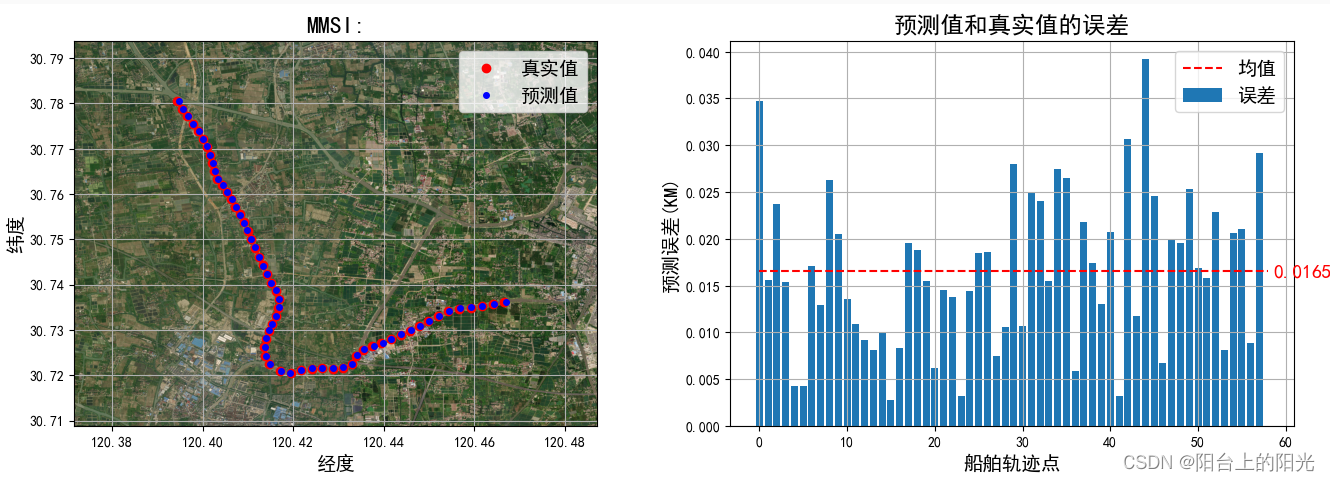
单步预测
test_points_ids = list(set(test['mmsi']))
for ids in test_points_ids[:1]:
y_pre = []
test_seq, test_label = createSequence(test.loc[test.mmsi == ids], windows, maxmin)
y_true = test_label
for i in range(len(test_seq)):
y_hat = model.predict(test_seq[i].reshape(1, windows, 4))
y_pre.append(y_hat[0])
y_pre = np.array(y_pre, dtype='float64')
# 反归一化
f_y_pre, f_y_true = FNormalizeMult(y_pre, y_true, maxmin)
print(f"最大值: {max(f_y_pre[:, 4])}\n最小值: {min(f_y_pre[:, 4])}\n均值: {np.mean(f_y_pre[:, 4])}\n"
f"方差: {np.var(f_y_pre[:, 4])}\n标准差: {np.std(f_y_pre[:, 4])}\n中位数: {np.median(f_y_pre[:, 4])}")
plt.figure(figsize=(16, 5))
plt.subplot(121)
plt.plot(f_y_true[:, 0], f_y_true[:, 1], "ro", markersize=6,label='真实值')
plt.plot(f_y_pre[:, 0], f_y_pre[:, 1], "bo",markersize=4, label='预测值')
bounds = [min(f_y_true[:, 0])-0.02,min(f_y_true[:, 1])-0.01,max(f_y_true[:, 0])+0.02,max(f_y_true[:, 1])+0.01]
tbd.plot_map(plt,bounds,zoom = 16,style = 3)
plt.legend(fontsize=14)
plt.grid()
plt.xlabel("经度",fontsize=14)
plt.ylabel("纬度",fontsize=14)
plt.title("MMSI:",fontsize=17)
meanss = np.mean(f_y_pre[:, 4])
plt.subplot(122)
plt.bar(range(f_y_pre.shape[0]),f_y_pre[:, 4],label='误差')
plt.plot([0,f_y_pre.shape[0]],[meanss,meanss],'--r',label="均值")
plt.title("预测值和真实值的误差",fontsize=17)
plt.xlabel("船舶轨迹点",fontsize=14)
plt.ylabel("预测误差(KM)",fontsize=14)
plt.text(f_y_pre.shape[0]*1.01,meanss*0.96,round(meanss,4),fontsize=14,color='r')
plt.grid()
plt.legend(fontsize=14)
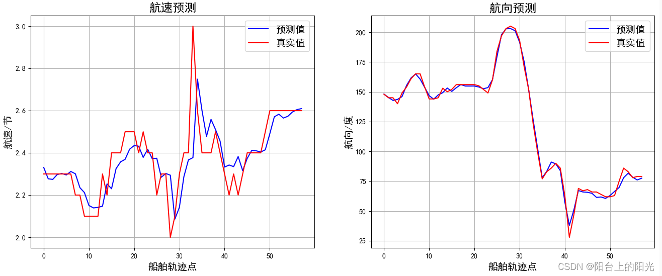
plt.figure(figsize=(16, 6))
plt.subplot(121)
plt.plot(f_y_pre[:, 2], "b-", label='预测值')
plt.plot(f_y_true[:, 2], "r-", label='真实值')
plt.legend(fontsize=14)
plt.title("航速预测",fontsize=17)
plt.xlabel("船舶轨迹点",fontsize=14)
plt.ylabel("航速/节",fontsize=14)
plt.grid()
plt.subplot(122)
plt.plot(f_y_pre[:, 3], "b-", label='预测值')
plt.plot(f_y_true[:, 3], "r-", label='真实值')
plt.legend(fontsize=14)
plt.title("航向预测",fontsize=17)
plt.xlabel("船舶轨迹点",fontsize=14)
plt.ylabel("航向/度",fontsize=14)
plt.grid()
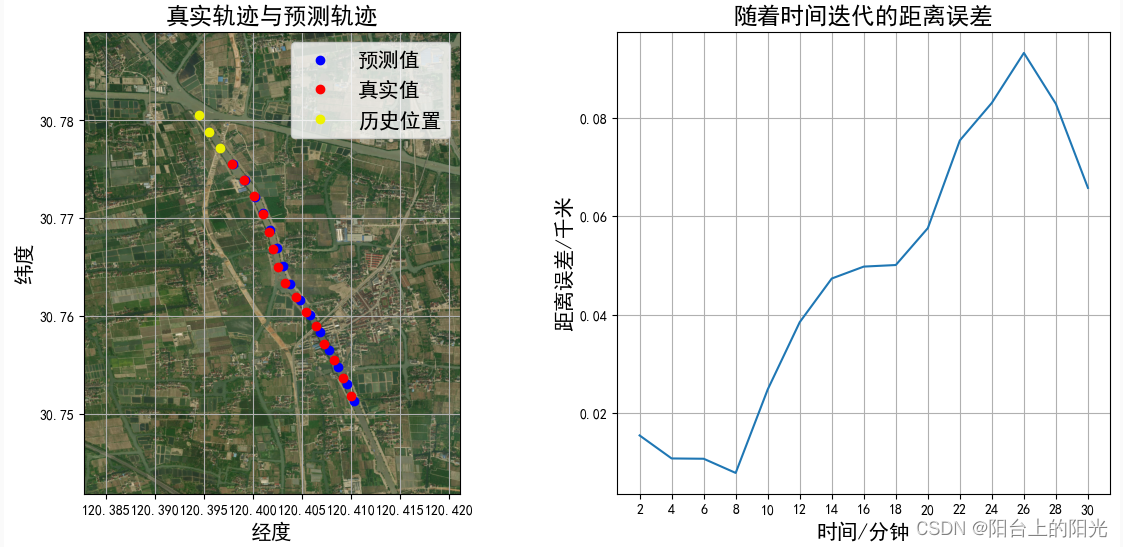
多步预测,船舶位置在最后一个黄色点位置
for ids in test_points_ids[:1]:
    test_seq, test_label = createSequence(test.loc[test.mmsi == ids], windows,maxmin)

    y_pre = []
    for i in range(len(test_seq)):
        y_hat = model.predict(test_seq[i].reshape(1, windows, 4))
        y_pre.append(y_hat[0])
    y_pre = np.array(y_pre, dtype='float64')
    # 得到真实值
    _,true_lables = FNormalizeMult(y_pre,np.copy(test_label),maxmin)

	# 从第四个开始预测
    for start_id in range(3,4):
        # 单值预测
        y_pre=[]
        y_true = []
        pre_seq = test_seq[start_id]
        # 最多预测 15 分钟
        maxStep = min(15,test_seq.shape[0] - start_id)
        # 循环预测
        for i in range(maxStep):
            y_hat = model.predict(pre_seq.reshape(1, windows, 4))
            y_pre.append(y_hat[0])
            y_true.append(test_label[start_id+i])
            # 下一个数组
            pre_seq = np.insert(pre_seq, pre_seq.shape[0], y_pre[i], axis=0)[1:]

        y_pre = np.array(y_pre, dtype='float64')
        y_true = np.array(y_true, dtype='float64')
        f_y_pre,f_y_true = FNormalizeMult(y_pre,y_true,maxmin)

        plt.figure(figsize=(14,6))
        plt.subplot(121)
        plt.plot(f_y_pre[:, 0], f_y_pre[:, 1], "bo", label='预测值')
        plt.plot(f_y_true[:, 0], f_y_true[:, 1], "ro", label='真实值')
        plt.plot(true_lables[:start_id, 0], true_lables[:start_id, 1], "o",color='#eef200', label='历史位置')
        bounds = [min(f_y_true[:, 0])-0.01,min(f_y_true[:, 1])-0.01,max(f_y_true[:, 0])+0.01,max(f_y_true[:, 1])+0.01]
        tbd.plot_map(plt,bounds,zoom = 16,style = 3)
        plt.legend(fontsize=15)
        plt.title(f'预测步数量={maxStep},开始位置={start_id}',fontsize=17)
        plt.title(f'真实轨迹与预测轨迹',fontsize=17)
        plt.xlabel("经度",fontsize=15)
        plt.ylabel("纬度",fontsize=15)
        plt.grid()

        plt.subplot(122)
        plt.plot(np.arange(2,2*(maxStep)+1,2),f_y_pre[:,4])
        plt.xticks(np.arange(2,2*(maxStep)+1,2))
        plt.title(f'随着时间迭代的距离误差',fontsize=17)
        plt.xlabel("时间/分钟",fontsize=15)
        plt.ylabel("距离误差/千米",fontsize=15)
        plt.grid()
        plt.show()
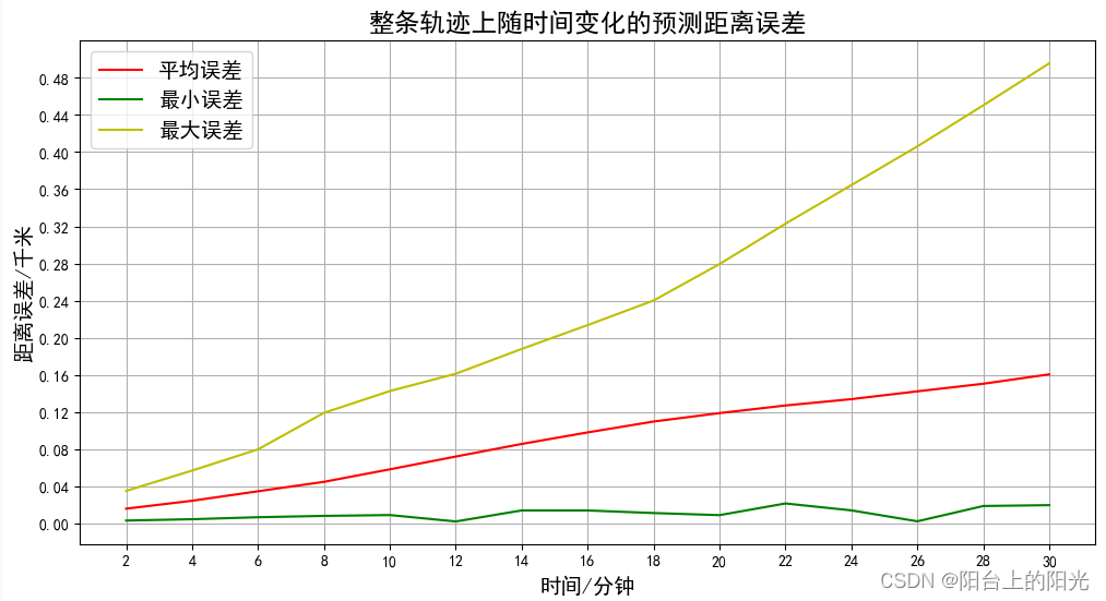
在整条轨迹上预测30分钟的误差
每个点都预测未来30分钟内的位置,然后把预测的某个时间(比如2分钟)的所有误差加到一起求均值
# 保存所有的预测误差
error_list = []
for ids in test_points_ids[:1]:
    test_seq, test_label = createSequence(test.loc[test.mmsi == ids], windows, maxmin)
    # 要预测的时间
    pre_time = 30
    for start_id in range(test_seq.shape[0]-int(pre_time/2)):
        # 单值预测
        y_pre=[]
        y_true = []
        pre_seq = test_seq[start_id]
        for i in range(int(pre_time/2)):
            y_hat = model.predict(pre_seq.reshape(1, windows, 4))
            y_pre.append(y_hat[0])
            y_true.append(test_label[start_id+i])
            # 下一个数组
            pre_seq = np.insert(pre_seq, pre_seq.shape[0], y_pre[i], axis=0)[1:]

        y_pre = np.array(y_pre, dtype='float64')
        y_true = np.array(y_true, dtype='float64')
        f_y_pre,f_y_true = FNormalizeMult(y_pre,y_true,maxmin)
        error_list.append(list(f_y_pre[:,4]))
b = np.zeros([len(error_list),len(max(error_list,key = lambda x: len(x)))])
for i,j in enumerate(error_list):
    b[i][0:len(j)] = j

sums = b.sum(axis=0)
maxx = b.max(axis=0)
minx = []
means = []
# 计算某个时间的预测误差的最值和均值
for col in range(b.shape[1]):
    fzeros = b.shape[0] - list(b[:,col]).count(0.0)
    minx.append(min(list(b[:fzeros,col])))
    means.append(sums[col] / fzeros)

plt.figure(figsize=(12,6))
plt.plot(np.arange(2,2*(b.shape[1])+1,2),means,'-r',label='平均误差')
plt.plot(np.arange(2,2*(b.shape[1])+1,2),minx,'-g',label='最小误差')
plt.plot(np.arange(2,2*(b.shape[1])+1,2),maxx,'-y',label='最大误差')
plt.xticks(np.arange(2,2*(b.shape[1])+1,2))
plt.yticks(np.arange(0,max(maxx),0.02))
plt.xlabel("时间/分钟",fontsize=14)
plt.ylabel("距离误差/千米",fontsize=14)
plt.legend(fontsize=14)
plt.grid()
plt.title("整条轨迹上随时间变化的预测距离误差",fontsize=17)
数据集及源码:
CSDN(免费): https://download.csdn.net/download/weixin_43261465/87526631
百度网盘:https://pan.baidu.com/s/1htJcYbmCgAh181SepREsiA 提取码: enpd


 595
595

 被折叠的 条评论
为什么被折叠?
被折叠的 条评论
为什么被折叠?
 到【灌水乐园】发言


