Learn_PyTorch_4_神经网络结构

1 神经网络基本结构

1.1 神经元

神经网络中，神经元模型如下：

用公式表示为：$$a=\sigma (z)=\sigma (a_1{w}_1+a_2{w}_2+\cdots +a_K{w}_K+b)$$
其中，$[a_1,...,a_k,...,a_K]$为神经元输入，$[w_1,...,w_k,...w_K]$为每个输入对应的权重，b为偏置，$\sigma (z)$为激活函数，$a$为神经元输出。

---

1.2 神经网络

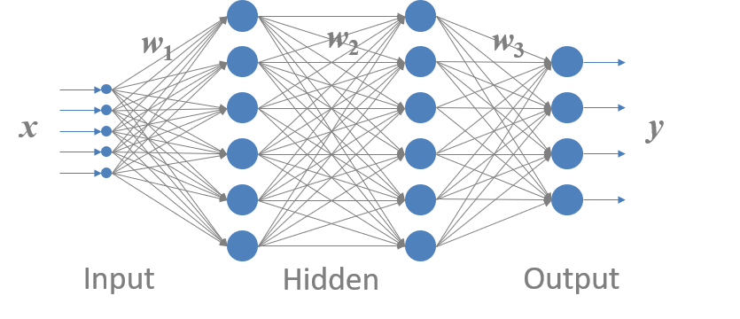
上图是一个典型的全连接神经网络结构，主要由输入层、隐含层和输出层构成。

其中， x = { x 1 , x 2 , . . . , x k } \boldsymbol x=\{x_1, x_2, ..., x_k\} x={x1​,x2​,...,xk​}为输入特征矢量，是神经网络的输入； y = { y 1 , y 2 , . . . , y d } \boldsymbol y=\{y_1, y_2, ..., y_d\} y={y1​,y2​,...,yd​}为神经网络的输出矢量； Θ = { W , b } \Theta = \{W, b\} Θ={W,b}为神经网络的参数，是神经网络训练过程所训练的对象。

下面以一个二分类问题来距离说明神经网络的基本结构和运行过程：

2 神经网络解决二分类问题

%matplotlib inline
import numpy as np
import matplotlib
import matplotlib.pyplot as plt
import torch
import torch.nn as nn
import torch.nn.functional as F
from torch.utils.data import Dataset, DataLoader

2.1 构造数据集

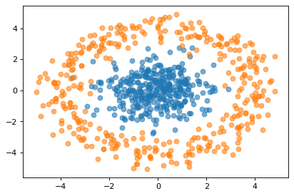
本文采用的数据集为随机产生的二维高斯分布离散点:

def rotate(theta):
    theta = theta  * np.pi / 180
    r = np.array([np.cos(theta), - np.sin(theta), np.sin(theta), np.cos(theta)]).reshape(2, 2)
    return r
x = np.random.multivariate_normal(mean = [0, 0], cov = [[1, 0], [0, 1]], size = 360)
y0 = np.array([4, 0]).reshape(2, 1)
y = np.array([rotate(theta).dot(y0) + np.random.randn(2).reshape(2, 1)/2 for theta in range(360)]).squeeze()

可视化如下：

plt.figure(dpi = 80)
plt.scatter(x[:, 0], x[:, 1], alpha = 0.6)
plt.scatter(y[:, 0], y[:, 1], alpha = 0.6)

构建数据集代码如下：

class dataSet(Dataset):
    """数据集"""
    
    def __init__(self, classA, classB, transform = None):
        self.data = torch.tensor(np.vstack((classA, classB)), dtype = torch.float)
        self.label = torch.cat((torch.zeros(len(classA), 1), torch.ones(len(classB), 1)))
        self.sample = torch.cat((self.data, self.label), 1)
    
    def __len__(self):
        return len(self.label)
    
    def __getitem__(self, idx):
        return self.sample[idx] # [x, y, label]

Data = dataSet(x, y) # 实例化数据集
dataLoader = DataLoader(Data, batch_size = 4) # 创建数据集迭代器，batch_size = 4

2.2 定义网络结构

对于二分类问题设计了如下简单的全连接神经网络：

定义的网络结构如下：

class LR(nn.Module):
    def __init__(self):
        super(LR, self).__init__()
        self.fc = nn.Linear(2, 5)
        self.fc1 = nn.Linear(5, 2)
        
    def forward(self, x):
        out = F.elu(self.fc(x))
        out = self.fc1(out)
        return out

其中，隐藏层fc将输入二维映射为5维(2 → 5)，激活函数使用的ELU（指数线性单元）；输出层fc1再将隐藏层输出的5维映射为2维，然后利用softmax函数对输出进行归一化，以便于分类。当y[0] > y[1]时，判定为a类，否则判定为b类。（后面会提到，当损失函数为交叉熵时输出层不加softmax函数进行归一化，因为PyTorch的CrossEntropyLoss自带softmax）

2.3 确定其他参数

2.3.1 损失函数

常用的损失函数主要由两个：均方误差和交叉熵。

其中，均方误差为：$$\text{MSE}=\frac{1}{2n}\sum _{i=1}^n(y_i-\widehat{y_i}{)}^2$$
交叉熵为：$$\text{CE}=-\sum _{i=1}^n{y}_i\ln \widehat{y_i}$$

对于分类问题来说，往往利用交叉熵作为损失函数，此时神经网络的输出层往往和分类的类别数相同，本例中为C = 2。

由于 { y 1 , y 2 , . . . , y n } \{y_1, y_2, ..., y_n\} {y1​,y2​,...,yn​}中只有一个为1，其它都为0， 因此交叉熵函数可以简化为：$$\text{CE}=-\ln \hat{y}$$

其中，$\hat{y}$为模型输出的估计值。当$\hat{y}$为1时，损失函数CE = 0；当$\hat{y}$趋于0时，损失函数CE趋于无穷大。

此外，PyTorch中的交叉熵损失函数集成了softmax函数，因此在CrossEntropyLoss中的源码可以看到，Pytorch中交叉熵损失函数的计算公式如下：

$$\text{loss}(x,class)=-\ln \left(\frac{\exp (x[class])}{{\sum }_j\exp (x[j])}\right)=-x[class]+\ln \left(\sum _j\exp (x[j])\right)$$
其中，$x$为神经网络输出层的输出（不含softmax)），class为样本的标记。如：

>>> output = torch.tensor([1, 2], dtype = torch.float).reshape(1, 2)
>>> label = torch.tensor([1], dtype = torch.long)
>>> criterion = torch.nn.CrossEntropyLoss()
>>> loss = criterion(output, label)
>>> loss
tensor(0.3133)

上述代码中， x = { 1 , 2 } ， class = 1 x = \{1, 2\}，\text{class} = 1 x={1,2}，class=1，代入$\text{loss}(x,lass)$中可得：$$\text{loss}(x,class)=-\ln (\frac{e^{x[1]}}{e^{x[0]}+e^{x[1]}})=-\ln (\frac{e^2}{e^1+e^2})=0.3133$$

值得注意的是，CrossEntropLoss要求输入的$x$数据类型为torch.float，而$\text{class}$的数据类型为torch.long

2.3.2 优化方法

常用的优化方法有Mini-batch SGD、Adadelta、Adam等，本例对优化方法的要求不高，因此选用Adam方法，它是一种自适应优化方法，基本不需要调参。

optim = torch.optim.Adam(net.parameters())

2.4 训练网络

完成上述操作之后，就可以开始训练神经网络了，如下：

epoches = 100 # 样本迭代次数（训练次数）
net = LR() # 实例化神经网络
optim = torch.optim.Adam(net.parameters()) # 实例化优化器，传入网络net的参数
for i in range(epoches): # 训练
    for idx, batch in enumerate(dataLoader): # Mini-batch
        data = batch[:, :2] # 前两列为数据
        label = batch[:, 2] # 第三列为标签
        yhat = net(data) # 正向传播
        loss = criterion(yhat, label.long()) # 计算损失
        optim.zero_grad() # 清空历史梯度
        loss.backward() # 计算当前梯度
        optim.step() # 更新参数
    if i % 10 == 0:
        print(loss) # 打印当前损失

输出：

tensor(0.4932, grad_fn=<NllLossBackward>)
tensor(0.0518, grad_fn=<NllLossBackward>)
tensor(0.0202, grad_fn=<NllLossBackward>)
tensor(0.0123, grad_fn=<NllLossBackward>)
tensor(0.0071, grad_fn=<NllLossBackward>)
tensor(0.0046, grad_fn=<NllLossBackward>)
tensor(0.0033, grad_fn=<NllLossBackward>)
tensor(0.0025, grad_fn=<NllLossBackward>)
tensor(0.0019, grad_fn=<NllLossBackward>)
tensor(0.0015, grad_fn=<NllLossBackward>)

可以看到，损失函数下降很快，当训练不到50次时，损失函数已经达到0.01以下。

2.5 可视化训练结果

利用matplotlib绘制出分类面如下：

可以看出，该网络很好的对两类数据进行了分类，在另一个同分布的测试样本集上的分类效果如下图所示：

可视化部分代码如下：

def visualization(net, x, y):
    x = np.linspace(-5, 5, 1000)
    y = np.linspace(-5, 5, 1000)
    X, Y = torch.tensor(np.meshgrid(a, b))
    point = torch.cat((X.unsqueeze(dim = 2), Y.unsqueeze(dim = 2)), dim = 2).reshape(-1, 2).float()
    out = net(point)
    val = (out[:, 1] > out[:, 0]) .reshape(1000, 1000)
    plt.figure(dip = 80)
    plt.scatter(x[:, 0], x[:, 1], alpha = 0.6)
    plt.scatter(y[:, 0], y[:, 1], alpha = 0.6)
    plt.contour(np.array(X), np.array(Y), val, colors = 'r' , alpha = 0.3)

完整代码见：https://github.com/WavenZ/Learn_PyTorch