我与机器学习 - [Today is AdaBoost] - [自适应分类器]

当作重要决定时，大家可能会考虑吸取多个专家的意见而不是只有一个人的意见。机器学习处理问题时何尝不是如此，这就是元算法背后的思路，元算法是对其他算法进行组合的一种方式。接下来我们将集中关注一个 AdaBoost的最流行的元算法。由于某些人认为这是最好的监督学习的方式，所以该方法是机器学习工具箱中最强有力的工具之一。

优点：泛化错误率低，易编码，可以应用在大部分的分类器上，无参数调整。

缺点：对离群点敏感。

适用数据类型：数值型和标称型。

bagging：基于数据随机重抽样的分类器构建方法

      自举汇聚法（bootstrap aggregating），也称为bagging方法，是在从原始数据集选择S次后得到S个新数据集的一种技术。新数据集和原始数据集大小相同。每个数据集都是通过原始数据集中随机选择一个样本来进行替换得到的。这里的替换就意味着可以多次的选择同一个样本，这一性质允许新数据集中可以有重复值，而原始数据集中的某些值在新的数据集中可能不会出现。

      在S个数据集构建好之后，将某个学习算法分别应用于每个数据集就得到了S个分类器。当我们要对新数据进行分类时，就可以应用这S个分类器进行分类，与此同时，选择分类器投票结果中最多的类别作为最后的分类结果。

boosting：

      boosting是一种与bagging很像的技术，不论是所使用的多个分类器的类型都是一致的，但是boosting中，不同的分类器是通过串行训练而获得的，每个新分类器都是根据已经训练处的分类器的性能来训练的。boosting是通过集中关注被已有分类器错分的那些数据来获得新的分类器，

      由于boosting分类的结果是基于所有分类器的加权和求结果的，因此boosting和bagging不大一样。bagging的分类器是权重相等的，而boosting中的分类器权重不同，每个权重代表的是其对应分类器在上一轮迭代中的成功度。

训练算法：基于错误提升分类器的性能

      能否使用弱分类器和多个实例来构建一个强分类器？这是一个非常有趣的理论问题。这里的“弱”意味着分类器的性能比随机猜测要略好，但是也不会好太多。这就是说，在二分类情况下弱分类器的错误率会高于50%，而“强”分类器的错误率将会低很多。AdaBoost算法即脱胎于上述理论问题。 
      AdaBoost是adaptive boosting（自适应boosting）的缩写，其运行过程如下：训练数据中的每个样本，并赋予其一个权重，这些权重构成了向量D。一开始，这些权重都初始化成相等值。首先在训练数据上训练出一个弱分类器并计算该分类器的错误率，然后在同一数据集上再次训练弱分类器。在分类器的第二次训练当中，将会重新调整每个样本的权重，其中第一次分对的样本的权重将会降低，而第一次分错的样本的权重将会提高。为了从所有弱分类器中得到最终的分类结果，AdaBoost为每个分类器都分配了一个权重值alpha，这些alpha值是基于每个弱分类器的错误率进行计算的。

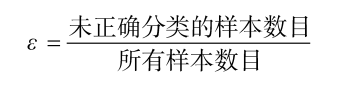
其中，错误率ε的定义为：

 

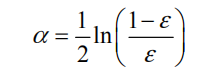
而alpha的计算公式如下：

 

AdaBoost算法的流程如图：

AdaBoost算法的示意图。左边是数据集，其中直方图的不同宽度表示每个样例上的不同权重。在经过一个分类器之后，加权的预测结果会通过三角形中的alpha值进行加权。每个三角形中输出的加权结果在圆形中求和，从而得到最终的输出结果 。

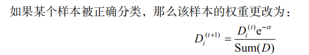
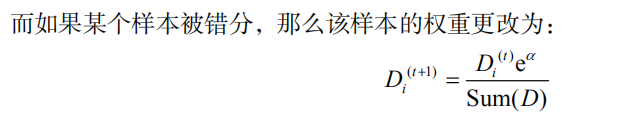
计算出alpha值之后，可以对权重向量D进行更新，以使得那些正确分类的样本的权重降低而错分样本的权重升高。

D的计算方法如下：

 

在计算出D之后，AdaBoost又开始进入下一轮迭代。AdaBoost算法会不断地重复训练和调整权重的过程，直到训练错误率为0或者弱分类器的数目达到用户的指定值为止。

下面来看具体的实现：

首先实现弱分类器，这里使用单层的决策树。

def stump_classify(data_matrix, dimen, thresh_val, thresh_ineq):
    ret_array = np.ones((np.shape(data_matrix)[0], 1))
    if thresh_ineq == 'lt':
        ret_array[data_matrix[:, dimen] <= thresh_val] = -1.0
    else:
        ret_array[data_matrix[:, dimen] > thresh_val] = -1.0
    return ret_array


def build_stump(data_mat, class_labels, D):
    data = np.mat(data_mat)
    labels = np.mat(class_labels).T
    m, n = np.shape(data)
    step_count = 10
    best_stump = {}
    best_class_est = np.mat(np.zeros((m, 1)))
    min_err = np.inf
    for i in range(n):
        range_min = data[:, i].min()
        range_max = data[:, i].max()
        step_size = (range_max - range_min) / step_count
        for j in range(-1, int(step_count) + 1):
            for inequel in ['lt', 'gt']:
                thresh_val = range_min + float(j) * step_size
                predicted_vals = stump_classify(data, i, thresh_val, inequel)
                err_arr = np.mat(np.ones((m, 1)))
                err_arr[predicted_vals == labels] = 0
                weight_err = D.T * err_arr
                print("split: dim %d, thresh: %.2f, thresh inequl: %s, the weight error is: %.3f" % (i, thresh_val, inequel, weight_err))
                if weight_err < min_err:
                    min_err = weight_err
                    best_class_est = predicted_vals.copy()
                    best_stump['dim'] = i
                    best_stump['thresh'] = thresh_val
                    best_stump['ineq'] = inequel
    return best_stump, min_err, best_class_est

      上述程序包含两个函数。第一个函数stumpClassify()是通过阈值比较对数据进行分类的。所有在阈值一边的数据会分到类别-1，而在另外一边的数据分到类别+1。该函数可以通过数组过滤来实现，首先将返回数组的全部元素设置为1，然后将所有不满足不等式要求的元素设置为-1。可以基于数据集中的任一元素进行比较，同时也可以将不等号在大于、小于之间切换。

      第二个函数buildStump()将会遍历stumpClassify()函数所有的可能输入值，并找到数据集上最佳的单层决策树。这里的“最佳”是基于数据的权重向量D来定义的，读者很快就会看到其具体定义了。在确保输入数据符合矩阵格式之后，整个函数就开始执行了。然后，函数将构建一个称为bestStump的空字典，这个字典用于存储给定权重向量D时所得到的最佳单层决策树的相关信息。变量numSteps用于在特征的所有可能值上进行遍历。而变量minError则在一开始就初始化成正无穷大，之后用于寻找可能的最小错误率。 
      三层嵌套的for循环是程序最主要的部分。第一层for循环在数据集的所有特征上遍历。考虑到数值型的特征，我们就可以通过计算最小值和最大值来了解应该需要多大的步长。然后，第二层for循环再在这些值上遍历。甚至将阈值设置为整个取值范围之外也是可以的。因此，在取值范围之外还应该有两个额外的步骤。最后一个for循环则是在大于和小于之间切换不等式。 
      在嵌套的三层for循环之内，我们在数据集及三个循环变量上调用stumpClassify()函数。基于这些循环变量，该函数将会返回分类预测结果。接下来构建一个列向量errArr，如果predictedVals中的值不等于labelMat中的真正类别标签值，那么errArr的相应位置为1。将错误向量errArr和权重向量D的相应元素相乘并求和，就得到了数值weightedError 。这就是AdaBoost和分类器交互的地方。这里，我们是基于权重向量D而不是其他错误计算指标来评价分类器的。如果需要使用其他分类器的话，就需要考虑D上最佳分类器所定义的计算过程。 
      程序接下来输出所有的值。最后，将当前的错误率与已有的最小错误率进行对比，如果当前的值较小，那么就在词典bestStump中保存该单层决策树。字典、错误率和类别估计值都会返回给AdaBoost算法。

接下来实现完整的adaboost：

def boost_train_ds(data_arr, class_labels, num_iter=40):
    week_class_arr = []
    m = np.shape(data_arr)[0]
    D = np.mat(np.ones((m, 1)) / m)
    agg_class_est = np.mat(np.zeros((m, 1)))
    for i in range(num_iter):
        best_stump, min_err, class_est = build_stump(data_arr, class_labels, D)
        print('D: ', D.T)
        print('error: ', min_err)
        alpha = float(0.5 * np.log((1.0 - min_err) / max(min_err, 1e-16)))
        print('alpha: ', alpha)
        best_stump['alpha'] = alpha
        week_class_arr.append(best_stump)
        print('class est:', class_est)
        expon = np.multiply(-1 * alpha * np.mat(class_labels).T, class_est)
        D = np.multiply(D, np.exp(expon))
        D = D / D.sum()
        agg_class_est += class_est * alpha
        print('aggclassest: ', agg_class_est)
        agg_error = np.multiply(np.sign(agg_class_est) != np.mat(class_labels).T, np.ones((m, 1)))
        error_rate = agg_error.sum() / m
        if error_rate == 0.0:
            break
    return week_class_arr

      AdaBoost算法的输入参数包括数据集、类别标签以及迭代次数numIt，其中numIt是在整个AdaBoost算法中唯一需要用户指定的参数。

      我们假定迭代次数设为9，如果算法在第三次迭代之后错误率为0，那么就会退出迭代过程，因此，此时就不需要执行所有的9次迭代过程。每次迭代的中间结果都会通过print语句进行输出。后面，读者可以把print输出语句注释掉，但是现在可以通过中间结果来了解AdaBoost算法的内部运行过程。

      函数名称尾部的DS代表的就是单层决策树（decision stump），它是AdaBoost中最流行的弱分类器，当然并非唯一可用的弱分类器。上述函数确实是建立于单层决策树之上的，但是我们也可以很容易对此进行修改以引入其他基分类器。实际上，任意分类器都可以作为基分类器，本书前面讲到的任何一个算法都行。上述算法会输出一个单层决策树的数组，因此首先需要建立一个新的Python表来对其进行存储。然后，得到数据集中的数据点的数目m，并建立一个列向量D。

      向量D非常重要，它包含了每个数据点的权重。一开始，这些权重都赋予了相等的值。在后续的迭代中，AdaBoost算法会在增加错分数据的权重的同时，降低正确分类数据的权重。D是一个概率分布向量，因此其所有的元素之和为1.0。为了满足此要求，一开始的所有元素都会被初始化成1/m。同时，程序还会建立另一个列向量aggClassEst，记录每个数据点的类别估计累计值。 

      AdaBoost算法的核心在于for循环，该循环运行numIt次或者直到训练错误率为0为止。循环中的第一件事就是利用前面介绍的buildStump()函数建立一个单层决策树。该函数的输入为权重向量D，返回的则是利用D而得到的具有最小错误率的单层决策树，同时返回的还有最小的错误率以及估计的类别向量。

      接下来，需要计算的则是alpha值。该值会告诉总分类器本次单层决策树输出结果的权重。其中的语句max(error, 1e-16)用于确保在没有错误时不会发生除零溢出。而后，alpha值加入到bestStump字典中，该字典又添加到列表中。该字典包括了分类所需要的所有信息。

      接下来的三行 则用于计算下一次迭代中的新权重向量D。在训练错误率为0时，就要提前结束for循环。此时程序是通过aggClassEst变量保持一个运行时的类别估计值来实现的 。该值只是一个浮点数，为了得到二值分类结果还需要调用sign()函数。如果总错误率为0，则由break语句中止for循环。

      接下来我们观察一下中间的运行结果。还记得吗，数据的类别标签为[1.0, 1.0, -1.0, -1.0, 1.0]。在第一轮迭代中，D中的所有值都相等。于是，只有第一个数据点被错分了。因此在第二轮迭代中，D向量给第一个数据点0.5的权重。这就可以通过变量aggClassEst的符号来了解总的类别。第二次迭代之后，我们就会发现第一个数据点已经正确分类了，但此时最后一个数据点却是错分了。D向量中的最后一个元素变成0.5，而D向量中的其他值都变得非常小。最后，第三次迭代之后aggClassEst所有值的符号和真实类别标签都完全吻合，那么训练错误率为0，程序就此退出。

程序输出：

E:\Anaconda\python.exe "E:/pycharm/PyCharm Community Edition 2018.2.3/bin/MLAProject/MLAProject/AdaBoost/adaboost.py"
split: dim 0, thresh: 0.90, thresh inequl: lt, the weight error is: 0.400
split: dim 0, thresh: 0.90, thresh inequl: gt, the weight error is: 0.600
split: dim 0, thresh: 1.00, thresh inequl: lt, the weight error is: 0.400
split: dim 0, thresh: 1.00, thresh inequl: gt, the weight error is: 0.600
split: dim 0, thresh: 1.10, thresh inequl: lt, the weight error is: 0.400
split: dim 0, thresh: 1.10, thresh inequl: gt, the weight error is: 0.600
split: dim 0, thresh: 1.20, thresh inequl: lt, the weight error is: 0.400
split: dim 0, thresh: 1.20, thresh inequl: gt, the weight error is: 0.600
split: dim 0, thresh: 1.30, thresh inequl: lt, the weight error is: 0.200
split: dim 0, thresh: 1.30, thresh inequl: gt, the weight error is: 0.800
split: dim 0, thresh: 1.40, thresh inequl: lt, the weight error is: 0.200
split: dim 0, thresh: 1.40, thresh inequl: gt, the weight error is: 0.800
split: dim 0, thresh: 1.50, thresh inequl: lt, the weight error is: 0.200
split: dim 0, thresh: 1.50, thresh inequl: gt, the weight error is: 0.800
split: dim 0, thresh: 1.60, thresh inequl: lt, the weight error is: 0.200
split: dim 0, thresh: 1.60, thresh inequl: gt, the weight error is: 0.800
split: dim 0, thresh: 1.70, thresh inequl: lt, the weight error is: 0.200
split: dim 0, thresh: 1.70, thresh inequl: gt, the weight error is: 0.800
split: dim 0, thresh: 1.80, thresh inequl: lt, the weight error is: 0.200
split: dim 0, thresh: 1.80, thresh inequl: gt, the weight error is: 0.800
split: dim 0, thresh: 1.90, thresh inequl: lt, the weight error is: 0.200
split: dim 0, thresh: 1.90, thresh inequl: gt, the weight error is: 0.800
split: dim 0, thresh: 2.00, thresh inequl: lt, the weight error is: 0.600
split: dim 0, thresh: 2.00, thresh inequl: gt, the weight error is: 0.400
split: dim 1, thresh: 0.89, thresh inequl: lt, the weight error is: 0.400
split: dim 1, thresh: 0.89, thresh inequl: gt, the weight error is: 0.600
split: dim 1, thresh: 1.00, thresh inequl: lt, the weight error is: 0.200
split: dim 1, thresh: 1.00, thresh inequl: gt, the weight error is: 0.800
split: dim 1, thresh: 1.11, thresh inequl: lt, the weight error is: 0.400
split: dim 1, thresh: 1.11, thresh inequl: gt, the weight error is: 0.600
split: dim 1, thresh: 1.22, thresh inequl: lt, the weight error is: 0.400
split: dim 1, thresh: 1.22, thresh inequl: gt, the weight error is: 0.600
split: dim 1, thresh: 1.33, thresh inequl: lt, the weight error is: 0.400
split: dim 1, thresh: 1.33, thresh inequl: gt, the weight error is: 0.600
split: dim 1, thresh: 1.44, thresh inequl: lt, the weight error is: 0.400
split: dim 1, thresh: 1.44, thresh inequl: gt, the weight error is: 0.600
split: dim 1, thresh: 1.55, thresh inequl: lt, the weight error is: 0.400
split: dim 1, thresh: 1.55, thresh inequl: gt, the weight error is: 0.600
split: dim 1, thresh: 1.66, thresh inequl: lt, the weight error is: 0.400
split: dim 1, thresh: 1.66, thresh inequl: gt, the weight error is: 0.600
split: dim 1, thresh: 1.77, thresh inequl: lt, the weight error is: 0.400
split: dim 1, thresh: 1.77, thresh inequl: gt, the weight error is: 0.600
split: dim 1, thresh: 1.88, thresh inequl: lt, the weight error is: 0.400
split: dim 1, thresh: 1.88, thresh inequl: gt, the weight error is: 0.600
split: dim 1, thresh: 1.99, thresh inequl: lt, the weight error is: 0.400
split: dim 1, thresh: 1.99, thresh inequl: gt, the weight error is: 0.600
split: dim 1, thresh: 2.10, thresh inequl: lt, the weight error is: 0.600
split: dim 1, thresh: 2.10, thresh inequl: gt, the weight error is: 0.400
D:  [[0.2 0.2 0.2 0.2 0.2]]
error:  [[0.2]]
alpha:  0.6931471805599453
class est: [[-1.]
 [ 1.]
 [-1.]
 [-1.]
 [ 1.]]
aggclassest:  [[-0.69314718]
 [ 0.69314718]
 [-0.69314718]
 [-0.69314718]
 [ 0.69314718]]
split: dim 0, thresh: 0.90, thresh inequl: lt, the weight error is: 0.250
split: dim 0, thresh: 0.90, thresh inequl: gt, the weight error is: 0.750
split: dim 0, thresh: 1.00, thresh inequl: lt, the weight error is: 0.625
split: dim 0, thresh: 1.00, thresh inequl: gt, the weight error is: 0.375
split: dim 0, thresh: 1.10, thresh inequl: lt, the weight error is: 0.625
split: dim 0, thresh: 1.10, thresh inequl: gt, the weight error is: 0.375
split: dim 0, thresh: 1.20, thresh inequl: lt, the weight error is: 0.625
split: dim 0, thresh: 1.20, thresh inequl: gt, the weight error is: 0.375
split: dim 0, thresh: 1.30, thresh inequl: lt, the weight error is: 0.500
split: dim 0, thresh: 1.30, thresh inequl: gt, the weight error is: 0.500
split: dim 0, thresh: 1.40, thresh inequl: lt, the weight error is: 0.500
split: dim 0, thresh: 1.40, thresh inequl: gt, the weight error is: 0.500
split: dim 0, thresh: 1.50, thresh inequl: lt, the weight error is: 0.500
split: dim 0, thresh: 1.50, thresh inequl: gt, the weight error is: 0.500
split: dim 0, thresh: 1.60, thresh inequl: lt, the weight error is: 0.500
split: dim 0, thresh: 1.60, thresh inequl: gt, the weight error is: 0.500
split: dim 0, thresh: 1.70, thresh inequl: lt, the weight error is: 0.500
split: dim 0, thresh: 1.70, thresh inequl: gt, the weight error is: 0.500
split: dim 0, thresh: 1.80, thresh inequl: lt, the weight error is: 0.500
split: dim 0, thresh: 1.80, thresh inequl: gt, the weight error is: 0.500
split: dim 0, thresh: 1.90, thresh inequl: lt, the weight error is: 0.500
split: dim 0, thresh: 1.90, thresh inequl: gt, the weight error is: 0.500
split: dim 0, thresh: 2.00, thresh inequl: lt, the weight error is: 0.750
split: dim 0, thresh: 2.00, thresh inequl: gt, the weight error is: 0.250
split: dim 1, thresh: 0.89, thresh inequl: lt, the weight error is: 0.250
split: dim 1, thresh: 0.89, thresh inequl: gt, the weight error is: 0.750
split: dim 1, thresh: 1.00, thresh inequl: lt, the weight error is: 0.125
split: dim 1, thresh: 1.00, thresh inequl: gt, the weight error is: 0.875
split: dim 1, thresh: 1.11, thresh inequl: lt, the weight error is: 0.250
split: dim 1, thresh: 1.11, thresh inequl: gt, the weight error is: 0.750
split: dim 1, thresh: 1.22, thresh inequl: lt, the weight error is: 0.250
split: dim 1, thresh: 1.22, thresh inequl: gt, the weight error is: 0.750
split: dim 1, thresh: 1.33, thresh inequl: lt, the weight error is: 0.250
split: dim 1, thresh: 1.33, thresh inequl: gt, the weight error is: 0.750
split: dim 1, thresh: 1.44, thresh inequl: lt, the weight error is: 0.250
split: dim 1, thresh: 1.44, thresh inequl: gt, the weight error is: 0.750
split: dim 1, thresh: 1.55, thresh inequl: lt, the weight error is: 0.250
split: dim 1, thresh: 1.55, thresh inequl: gt, the weight error is: 0.750
split: dim 1, thresh: 1.66, thresh inequl: lt, the weight error is: 0.250
split: dim 1, thresh: 1.66, thresh inequl: gt, the weight error is: 0.750
split: dim 1, thresh: 1.77, thresh inequl: lt, the weight error is: 0.250
split: dim 1, thresh: 1.77, thresh inequl: gt, the weight error is: 0.750
split: dim 1, thresh: 1.88, thresh inequl: lt, the weight error is: 0.250
split: dim 1, thresh: 1.88, thresh inequl: gt, the weight error is: 0.750
split: dim 1, thresh: 1.99, thresh inequl: lt, the weight error is: 0.250
split: dim 1, thresh: 1.99, thresh inequl: gt, the weight error is: 0.750
split: dim 1, thresh: 2.10, thresh inequl: lt, the weight error is: 0.750
split: dim 1, thresh: 2.10, thresh inequl: gt, the weight error is: 0.250
D:  [[0.5   0.125 0.125 0.125 0.125]]
error:  [[0.125]]
alpha:  0.9729550745276565
class est: [[ 1.]
 [ 1.]
 [-1.]
 [-1.]
 [-1.]]
aggclassest:  [[ 0.27980789]
 [ 1.66610226]
 [-1.66610226]
 [-1.66610226]
 [-0.27980789]]
split: dim 0, thresh: 0.90, thresh inequl: lt, the weight error is: 0.143
split: dim 0, thresh: 0.90, thresh inequl: gt, the weight error is: 0.857
split: dim 0, thresh: 1.00, thresh inequl: lt, the weight error is: 0.357
split: dim 0, thresh: 1.00, thresh inequl: gt, the weight error is: 0.643
split: dim 0, thresh: 1.10, thresh inequl: lt, the weight error is: 0.357
split: dim 0, thresh: 1.10, thresh inequl: gt, the weight error is: 0.643
split: dim 0, thresh: 1.20, thresh inequl: lt, the weight error is: 0.357
split: dim 0, thresh: 1.20, thresh inequl: gt, the weight error is: 0.643
split: dim 0, thresh: 1.30, thresh inequl: lt, the weight error is: 0.286
split: dim 0, thresh: 1.30, thresh inequl: gt, the weight error is: 0.714
split: dim 0, thresh: 1.40, thresh inequl: lt, the weight error is: 0.286
split: dim 0, thresh: 1.40, thresh inequl: gt, the weight error is: 0.714
split: dim 0, thresh: 1.50, thresh inequl: lt, the weight error is: 0.286
split: dim 0, thresh: 1.50, thresh inequl: gt, the weight error is: 0.714
split: dim 0, thresh: 1.60, thresh inequl: lt, the weight error is: 0.286
split: dim 0, thresh: 1.60, thresh inequl: gt, the weight error is: 0.714
split: dim 0, thresh: 1.70, thresh inequl: lt, the weight error is: 0.286
split: dim 0, thresh: 1.70, thresh inequl: gt, the weight error is: 0.714
split: dim 0, thresh: 1.80, thresh inequl: lt, the weight error is: 0.286
split: dim 0, thresh: 1.80, thresh inequl: gt, the weight error is: 0.714
split: dim 0, thresh: 1.90, thresh inequl: lt, the weight error is: 0.286
split: dim 0, thresh: 1.90, thresh inequl: gt, the weight error is: 0.714
split: dim 0, thresh: 2.00, thresh inequl: lt, the weight error is: 0.857
split: dim 0, thresh: 2.00, thresh inequl: gt, the weight error is: 0.143
split: dim 1, thresh: 0.89, thresh inequl: lt, the weight error is: 0.143
split: dim 1, thresh: 0.89, thresh inequl: gt, the weight error is: 0.857
split: dim 1, thresh: 1.00, thresh inequl: lt, the weight error is: 0.500
split: dim 1, thresh: 1.00, thresh inequl: gt, the weight error is: 0.500
split: dim 1, thresh: 1.11, thresh inequl: lt, the weight error is: 0.571
split: dim 1, thresh: 1.11, thresh inequl: gt, the weight error is: 0.429
split: dim 1, thresh: 1.22, thresh inequl: lt, the weight error is: 0.571
split: dim 1, thresh: 1.22, thresh inequl: gt, the weight error is: 0.429
split: dim 1, thresh: 1.33, thresh inequl: lt, the weight error is: 0.571
split: dim 1, thresh: 1.33, thresh inequl: gt, the weight error is: 0.429
split: dim 1, thresh: 1.44, thresh inequl: lt, the weight error is: 0.571
split: dim 1, thresh: 1.44, thresh inequl: gt, the weight error is: 0.429
split: dim 1, thresh: 1.55, thresh inequl: lt, the weight error is: 0.571
split: dim 1, thresh: 1.55, thresh inequl: gt, the weight error is: 0.429
split: dim 1, thresh: 1.66, thresh inequl: lt, the weight error is: 0.571
split: dim 1, thresh: 1.66, thresh inequl: gt, the weight error is: 0.429
split: dim 1, thresh: 1.77, thresh inequl: lt, the weight error is: 0.571
split: dim 1, thresh: 1.77, thresh inequl: gt, the weight error is: 0.429
split: dim 1, thresh: 1.88, thresh inequl: lt, the weight error is: 0.571
split: dim 1, thresh: 1.88, thresh inequl: gt, the weight error is: 0.429
split: dim 1, thresh: 1.99, thresh inequl: lt, the weight error is: 0.571
split: dim 1, thresh: 1.99, thresh inequl: gt, the weight error is: 0.429
split: dim 1, thresh: 2.10, thresh inequl: lt, the weight error is: 0.857
split: dim 1, thresh: 2.10, thresh inequl: gt, the weight error is: 0.143
D:  [[0.28571429 0.07142857 0.07142857 0.07142857 0.5       ]]
error:  [[0.14285714]]
alpha:  0.8958797346140273
class est: [[1.]
 [1.]
 [1.]
 [1.]
 [1.]]
aggclassest:  [[ 1.17568763]
 [ 2.56198199]
 [-0.77022252]
 [-0.77022252]
 [ 0.61607184]]
[{'dim': 0, 'thresh': 1.3, 'ineq': 'lt', 'alpha': 0.6931471805599453}, {'dim': 1, 'thresh': 1.0, 'ineq': 'lt', 'alpha': 0.9729550745276565}, {'dim': 0, 'thresh': 0.9, 'ineq': 'lt', 'alpha': 0.8958797346140273}]

Process finished with exit code 0

以上便是adaboost算法的实现部分，下面我们来看下怎么做预测。

def ada_classify(data_to_class, classifyer):
    data = np.mat(data_to_class)
    m = np.shape(data)[0]
    agg_class_est = np.mat(np.zeros((m, 1)))
    for i in range(len(classifyer)):
        class_est = stump_classify(data, classifyer[i]['dim'], classifyer[i]['thresh'], classifyer[i]['ineq'])
        agg_class_est += class_est * classifyer[i]['alpha']
        print(agg_class_est)
        return np.sign(agg_class_est)

预测无外乎就是对训练得到的所有若分类器加权求和。

以上部分的代码：https://github.com/HanGaaaaa/MLAProject/tree/master/AdaBoost