


空间四点定位原理与实现
文章目录
前言
前文中实现了平面中三点定位及相关应用,本文在此基础上利用其原理在空间中实现四点定位和相关应用。文章涉及代码放在以下链接中:
链接:https://pan.baidu.com/s/1u9ZgR_gXU2VeEokEpW-cIA 或 所用代码链接
提取码:wv53
一、空间四点定位原理
1.原理推导
已知空间内四点和它们到任意一点的距离,则可以通过距离关系得到四个二次等式,在通过三组差分消去高次项后得到方程组,通过矩阵运算解出任意一点的坐标。
假设空间中已知四点A、B、C、D,坐标分别为
(
x
1
,
y
1
)
(x_{1},y_{1})
(x1,y1)、
(
x
2
,
y
2
)
(x_{2},y_{2})
(x2,y2)、
(
x
3
,
y
3
)
(x_{3},y_{3})
(x3,y3)、
(
x
4
,
y
4
)
(x_{4},y_{4})
(x4,y4),一待定位点P坐标为
(
x
,
y
)
(x,y)
(x,y),P到四点的距离分别为
ρ
1
,
ρ
2
,
ρ
3
,
ρ
4
\rho_{1},\rho_{2},\rho_{3},\rho_{4}
ρ1,ρ2,ρ3,ρ4,根据距离公式,可以得到一个如下的方程组:
{
(
x
1
−
x
)
2
+
(
y
1
−
y
)
2
+
(
z
1
−
z
)
2
=
ρ
1
2
(
x
2
−
x
)
2
+
(
y
2
−
y
)
2
+
(
z
2
−
z
)
2
=
ρ
2
2
(
x
3
−
x
)
2
+
(
y
3
−
y
)
2
+
(
z
3
−
z
)
2
=
ρ
3
2
(
x
4
−
x
)
2
+
(
y
4
−
y
)
2
+
(
z
4
−
z
)
2
=
ρ
4
2
\begin{cases} (x_{1}-x)^2+(y_{1}-y)^2+(z_{1}-z)^2=\rho_{1}^2 \\ (x_{2}-x)^2+(y_{2}-y)^2+(z_{2}-z)^2=\rho_{2}^2 \\ (x_{3}-x)^2+(y_{3}-y)^2+(z_{3}-z)^2=\rho_{3}^2\\ (x_{4}-x)^2+(y_{4}-y)^2+(z_{4}-z)^2=\rho_{4}^2 \end{cases}
⎩⎪⎪⎪⎨⎪⎪⎪⎧(x1−x)2+(y1−y)2+(z1−z)2=ρ12(x2−x)2+(y2−y)2+(z2−z)2=ρ22(x3−x)2+(y3−y)2+(z3−z)2=ρ32(x4−x)2+(y4−y)2+(z4−z)2=ρ42
进行整理得到:
{
x
2
−
2
x
1
x
+
y
2
−
2
y
1
y
+
z
2
−
2
z
1
z
=
ρ
1
2
−
x
1
2
−
y
1
2
−
z
1
2
x
2
−
2
x
2
x
+
y
2
−
2
y
2
y
+
z
2
−
2
z
2
z
=
ρ
2
2
−
x
2
2
−
y
2
2
−
z
2
2
x
2
−
2
x
3
x
+
y
2
−
2
y
3
y
+
z
2
−
2
z
3
z
=
ρ
3
2
−
x
3
2
−
y
3
2
−
z
3
2
x
2
−
2
x
4
x
+
y
2
−
2
y
4
y
+
z
2
−
2
z
4
z
=
ρ
4
2
−
x
4
2
−
y
4
2
−
z
4
2
\begin{cases} x^2-2x_{1}x+y^2-2y_{1}y+z^2-2z_{1}z=\rho_{1}^2-x_{1}^{2}- y_{1}^{2}-z_{1}^2\\ x^2-2x_{2}x+y^2-2y_{2}y+z^2-2z_{2}z=\rho_{2}^2-x_{2}^{2}- y_{2}^{2}-z_{2}^2 \\ x^2-2x_{3}x+y^2-2y_{3}y+z^2-2z_{3}z=\rho_{3}^2-x_{3}^{2}- y_{3}^{2}-z_{3}^2 \\ x^2-2x_{4}x+y^2-2y_{4}y+z^2-2z_{4}z=\rho_{4}^2-x_{4}^{2}- y_{4}^{2}-z_{4}^2 \end{cases}
⎩⎪⎪⎪⎨⎪⎪⎪⎧x2−2x1x+y2−2y1y+z2−2z1z=ρ12−x12−y12−z12x2−2x2x+y2−2y2y+z2−2z2z=ρ22−x22−y22−z22x2−2x3x+y2−2y3y+z2−2z3z=ρ32−x32−y32−z32x2−2x4x+y2−2y4y+z2−2z4z=ρ42−x42−y42−z42
可以看出上式中含有高次项,不利于方程的求解,而对方程进行三次差分可以消除掉高次项,得到以下的一次方程组:
{
2
x
(
x
2
−
x
1
)
+
2
y
(
y
2
−
y
1
)
+
2
z
(
z
2
−
z
1
)
=
ρ
1
2
−
ρ
2
2
+
x
2
2
−
x
1
2
+
y
2
2
−
y
1
2
+
z
2
2
−
z
1
2
2
x
(
x
3
−
x
1
)
+
2
y
(
y
3
−
y
1
)
+
2
z
(
z
3
−
z
1
)
=
ρ
1
2
−
ρ
3
2
+
x
3
2
−
x
1
2
+
y
3
2
−
y
1
2
+
z
3
2
−
z
1
2
2
x
(
x
4
−
x
1
)
+
2
y
(
y
4
−
y
1
)
+
2
z
(
z
4
−
z
1
)
=
ρ
1
2
−
ρ
4
2
+
x
4
2
−
x
1
2
+
y
4
2
−
y
1
2
+
z
4
2
−
z
1
2
\begin{cases} 2x(x_{2}-x_{1})+2y(y_{2}-y_{1})+2z(z_{2}-z_{1})=\rho_{1}^2-\rho_{2}^2+x_{2}^{2}-x_{1}^{2}+y_{2}^{2}-y_{1}^{2}+z_{2}^2-z_{1}^2\\ 2x(x_{3}-x_{1})+2y(y_{3}-y_{1})+2z(z_{3}-z_{1})=\rho_{1}^2-\rho_{3}^2+x_{3}^{2}-x_{1}^{2}+y_{3}^{2}-y_{1}^{2}+z_{3}^2-z_{1}^2\\ 2x(x_{4}-x_{1})+2y(y_{4}-y_{1})+2z(z_{4}-z_{1})=\rho_{1}^2-\rho_{4}^2+x_{4}^{2}-x_{1}^{2}+y_{4}^{2}-y_{1}^{2}+z_{4}^2-z_{1}^2 \end{cases}
⎩⎪⎨⎪⎧2x(x2−x1)+2y(y2−y1)+2z(z2−z1)=ρ12−ρ22+x22−x12+y22−y12+z22−z122x(x3−x1)+2y(y3−y1)+2z(z3−z1)=ρ12−ρ32+x32−x12+y32−y12+z32−z122x(x4−x1)+2y(y4−y1)+2z(z4−z1)=ρ12−ρ42+x42−x12+y42−y12+z42−z12
将方程式用矩阵形式表示,
A
c
=
b
\mathrm{A}c=b
Ac=b
其中
A
=
[
2
(
x
2
−
x
1
)
2
(
y
2
−
y
1
)
)
2
(
z
2
−
z
1
)
2
(
x
3
−
x
1
)
2
(
y
3
−
y
1
)
)
2
(
z
3
−
z
1
)
2
(
x
4
−
x
1
)
2
(
y
4
−
y
1
)
)
2
(
z
4
−
z
1
)
]
\mathrm{A}=\begin{bmatrix} 2(x_{2}-x_{1})&2(y_{2}-y_{1}))&2(z_{2}-z_{1})\\ 2(x_{3}-x_{1})&2(y_{3}-y_{1}))&2(z_{3}-z_{1})\\ 2(x_{4}-x_{1})&2(y_{4}-y_{1}))&2(z_{4}-z_{1}) \end{bmatrix}
A=⎣⎡2(x2−x1)2(x3−x1)2(x4−x1)2(y2−y1))2(y3−y1))2(y4−y1))2(z2−z1)2(z3−z1)2(z4−z1)⎦⎤
c
=
(
x
y
z
)
c=\begin{pmatrix} x\\ y\\ z \end{pmatrix}
c=⎝⎛xyz⎠⎞
b
=
(
ρ
1
2
−
ρ
2
2
+
x
2
2
−
x
1
2
+
y
2
2
−
y
1
2
+
z
2
2
−
z
1
2
ρ
1
2
−
ρ
3
2
+
x
3
2
−
x
1
2
+
y
3
2
−
y
1
2
+
z
3
2
−
z
1
2
ρ
1
2
−
ρ
4
2
+
x
4
2
−
x
1
2
+
y
4
2
−
y
1
2
+
z
4
2
−
z
1
2
)
b=\begin{pmatrix} \rho_{1}^2-\rho_{2}^2+x_{2}^{2}-x_{1}^{2}+y_{2}^{2}-y_{1}^{2}+z_{2}^2-z_{1}^2\\ \rho_{1}^2-\rho_{3}^2+x_{3}^{2}-x_{1}^{2}+y_{3}^{2}-y_{1}^{2}+z_{3}^2-z_{1}^2\\ \rho_{1}^2-\rho_{4}^2+x_{4}^{2}-x_{1}^{2}+y_{4}^{2}-y_{1}^{2}+z_{4}^2-z_{1}^2 \end{pmatrix}
b=⎝⎛ρ12−ρ22+x22−x12+y22−y12+z22−z12ρ12−ρ32+x32−x12+y32−y12+z32−z12ρ12−ρ42+x42−x12+y42−y12+z42−z12⎠⎞
由矩阵的运算可见,要求得待定位点坐标
(
x
,
y
)
(x,y)
(x,y),也就是求解向量
c
c
c,如果矩阵
A
\mathrm{A}
A的逆矩阵存在,由下式即可求解出向量
c
c
c:
c
=
A
−
1
b
c=\mathrm{A}^{-1}b
c=A−1b
到此为止,待求解点的坐标已经可以解算出,这要求我们在选取已知点时保证矩阵
A
\mathrm{A}
A的可逆性,从几何上看需保证已知四点不在同一平面内。
二、Matlab代码实现
1.画球程序
为了体现原理,需要在已知球心处按一定半径画球,因此首先实现画球程序
function h=DrawSphere(r,x0,y0,z0)
%DrawSphere function draw a sphere which has radius r and center (x0,y0,z0)

[x,y,z]=sphere(30);

%调整半径
x=r*x;
y=r*y;
z=r*z;

%调整圆心
x=x+x0;
y=y+y0;
z=z+z0;

% hold on;
% axis equal;
% mesh(x,y,z);


axis equal;
s = surf(x,y,z,'FaceAlpha',0.3);
s.EdgeColor = 'none';
hold on;

%hold on;
%axis equal;
%plot3(x,y,z);
2.主程序
2.1 空间中随机取一点作为待定位点
首先需要将四个已知坐标点的坐标保存并在坐标系中绘制出,之后获取几个待定位点的坐标,用于计算距离和最终与解算点作对比,通过 t a r g e t = 100 ∗ r a n d ( 1 , 3 ) ; target = 100*rand(1,3); target=100∗rand(1,3);,在空间坐标系中确定一点作为待定位点。
clear all
disp('Four points Mesurement')
x = [0,0,0,50];
y = [0,0,50,50];
z = [0,50,0,50];
figure('Name','空间四点定位图','NumberTitle','off');
plot3(x,y,z,'o');
xlabel('x坐标/m');
ylabel('y坐标/m');
zlabel('z坐标/m');
axis([-5,100,-5,100,-5,100]);
hold on
target = 100*rand(1,3);
x0=target(1);
y0=target(2);
z0=target(3);
plot3(x0,y0,z0,'k:o');
axis([-5,100,-5,100,-5,100]);
2.2 距离计算
通过距离公式可以获得待定位点到四个已知位置点的距离,这在伪距定位中对应卫星和地面待测点之间的伪距,通过对距离加入误差,进而观察最终的定位精度可以模拟伪距定位过程中各因素对最终定位结果产生的影响。
distance=zeros(1,4);
for j=1:4
  distance(j)=sqrt((x0-x(j))^2+(y0-y(j))^2+(z0-z(j))^2);
end
% random_error=rand(1,4)-0.3;%加入随机误差
% bias_error = 0.05*distance;
% distance=distance-distance.*(random_error/7) + bias_error;
2.3 坐标解算
通过一中原理推导,只需要简单的矩阵运算就可以解算出待定位点坐标
A = zeros(3);
b = zeros(3,1);
c = zeros(3,1);

for h=1;1
    A = 2*([x(2)-x(1),y(2)-y(1),z(2)-z(1);
                x(3)-x(1),y(3)-y(1),z(3)-z(1);
                x(4)-x(1),y(4)-y(1),z(4)-z(1)])

    A = inv(A);

    b = [distance(1)^2-distance(2)^2+x(2)^2-x(1)^2+y(2)^2-y(1)^2+z(2)^2-z(1)^2;
        distance(1)^2-distance(3)^2+x(3)^2-x(1)^2+y(3)^2-y(1)^2+z(3)^2-z(1)^2;
        distance(1)^2-distance(4)^2+x(4)^2-x(1)^2+y(4)^2-y(1)^2+z(4)^2-z(1)^2]
    c = A*b;%实际坐标
    plot3(c(1),c(2),c(3),'k:+');
    axis([-5,120,-5,120,-5,120])
    DrawSphere(distance(1),x(1),y(1),z(1));
    DrawSphere(distance(2),x(2),y(2),z(2));
    DrawSphere(distance(3),x(3),y(3),z(3));
    DrawSphere(distance(4),x(4),y(4),z(4));
    plot3([x(1),c(1)],[y(1),c(2)],[z(1),c(3)],'k');
    plot3([x(2),c(1)],[y(2),c(2)],[z(2),c(3)],'k');
    plot3([x(3),c(1)],[y(3),c(2)],[z(3),c(3)],'k');
    plot3([x(4),c(1)],[y(4),c(2)],[z(4),c(3)],'k');
    axis([-50,100,-50,100,-50,100]);
    grid on;
end
通过主程序代码可以实现空间中四点定位原理的示意。
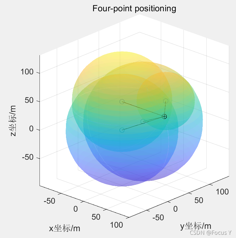
在空间中随机确定一点,以上图片为输出例子,图中深色圆圈为圆之间的交点,+号的点为开始用鼠标在坐标系中确定的点,可以发现两者是完全重合的,证明空间四点定位算法原理的正确性。
3.误差分析
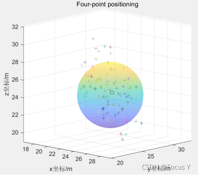
主程序中的例子是为了说明四点定位的原理,实际意义有限,毕竟某种程度上来说是已知答案推过程。为了实际性,对空间四点定位的误差进行分析,在主程序的基础上加入干扰,多次定位同一点,观察误差情况。
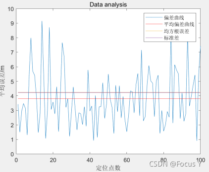
误差评定指标:
1.平均偏差:定位点与待定位点距离的平均值,反映定位精确度
2.均方根误差:反映定位精确度

3.标准差:反映定位精密度

4.SEP球概率
指以平均坐标为球心,使50%点落在球内的半径,SEP越小代表定位精度越高。
C
E
P
=
0.51
(
δ
x
+
δ
y
+
δ
z
)
CEP=0.51(\delta_{x}+\delta_{y}+\delta_{z})
CEP=0.51(δx+δy+δz)
δ
x
,
δ
y
,
δ
z
\delta_{x},\delta_{y},\delta_{z}
δx,δy,δz指点集所有点的
x
,
y
,
z
x,y,z
x,y,z坐标标准差。
clear all
disp('Four points Mesurement')
x = [0,0,0,50];
y = [0,0,50,50];
z = [0,50,0,50];
figure('Name','空间四点定位图','NumberTitle','off');
plot3(x,y,z,'o');
xlabel('x坐标/m');
ylabel('y坐标/m');
zlabel('z坐标/m');
axis([-5,100,-5,100,-5,100]);
hold on
%target = 100*rand(1,3);
x0=25*ones(1,100);
y0=25*ones(1,100);
z0=25*ones(1,100);
plot3(x0,y0,z0,'k:o');
axis([-5,100,-5,100,-5,100]);

distance=zeros(1,4,100);
for j=1:4
    for h=1:100
        distance(1,j,h)=sqrt((x0(h)-x(j))^2+(y0(h)-y(j))^2+(z0(h)-z(j))^2);
    end
end

random_error=rand(1,4,100)-0.3;
bias_error = 0.05*distance;
distance=distance-distance.*(random_error/7) + bias_error;      %误差控制?

A = zeros(3,3,100);
b = zeros(3,1,100);
c = zeros(3,1,100);

for k=1:100
    A(:,:,k) = 2*([x(2)-x(1),y(2)-y(1),z(2)-z(1);
                x(3)-x(1),y(3)-y(1),z(3)-z(1);
                x(4)-x(1),y(4)-y(1),z(4)-z(1)]);

    A(:,:,k) = inv(A(:,:,k));

    b(:,:,k) = [distance(1,1,k)^2-distance(1,2,k)^2+x(2)^2-x(1)^2+y(2)^2-y(1)^2+z(2)^2-z(1)^2;
        distance(1,1,k)^2-distance(1,3,k)^2+x(3)^2-x(1)^2+y(3)^2-y(1)^2+z(3)^2-z(1)^2;
        distance(1,1,k)^2-distance(1,4,k)^2+x(4)^2-x(1)^2+y(4)^2-y(1)^2+z(4)^2-z(1)^2];
    c(:,:,k) = A(:,:,k)*b(:,:,k);%实际坐标
    plot3(c(1,1,k),c(2,1,k),c(3,1,k),'color',[rand rand rand],'Marker','+');
    axis([-5,120,-5,120,-5,120]);
%     DrawSphere(distance(1),x(1),y(1),z(1));
%     DrawSphere(distance(2),x(2),y(2),z(2));
%     DrawSphere(distance(3),x(3),y(3),z(3));
%     DrawSphere(distance(4),x(4),y(4),z(4));
%     plot3([x(1),c(1)],[y(1),c(2)],[z(1),c(3)],'k');
%     plot3([x(2),c(1)],[y(2),c(2)],[z(2),c(3)],'k');
%     plot3([x(3),c(1)],[y(3),c(2)],[z(3),c(3)],'k');
%     plot3([x(4),c(1)],[y(4),c(2)],[z(4),c(3)],'k');
    grid on;
end

%计算误差
%1.平均偏差
loop_index = 1:100;
distance_error = sqrt((c(1,:,:)-25).^2+(c(2,:,:)-25).^2+(c(3,:,:)-25).^2);
mean_error = mean(distance_error);

%2.均方根误差
RMSE = sqrt(mean((c(1,:,:)-25).^2+(c(2,:,:)-25).^2+(c(3,:,:)-25).^2));
%3.标准差
mean_position = mean(c,3);
std_error = sqrt(mean((c(1,:,:)-mean_position(1)).^2+(c(2,:,:)-mean_position(2)).^2+(c(3,:,:)-mean_position(3)).^2,3));
%4.CEP圆概率
std_x = sqrt(mean((c(1,:,:)-mean_position(1)).^2));
std_y = sqrt(mean((c(2,:,:)-mean_position(2)).^2));
std_z = sqrt(mean((c(3,:,:)-mean_position(3)).^2));
SEP = 0.51*(std_x+std_y+std_z);
figure(1);
DrawSphere(SEP,mean_position(1),mean_position(2),mean_position(3));

%画误差图
figure('Name','误差分析图','NumberTitle','off');
plot([1:100],squeeze(squeeze(distance_error)),[1:100],mean_error*ones(1,100),'r',[1:100],RMSE*ones(1,100),[1:100],std_error*ones(1,100)),legend('偏差曲线','平均偏差曲线','均方根误差','标准差');
xlabel('定位点数');
ylabel('平均误差/m');
ss = 'Data analysis';
title(ss);
s='Four-point positioning';
figure(1);
title(s);
以下是程序运行的结果:
4.动态轨迹跟踪
前文实现了单点和多点定位,而一点的运动轨迹可以分解为多个点的集合,因此既然能实现单点定位,也能实现轨迹跟踪。在单点和多点定位的基础上,分别加入误差和不加入误差,对空间内一运动点的轨迹进行跟踪。
clear all
disp('Four points Mesurement')
x = [0,0,0,50];
y = [0,0,50,50];
z = [0,50,0,50];
s='Four-point positioning';
figure('Name','空间四点定位图','NumberTitle','off');
plot3(x,y,z,'o');
xlabel('x坐标/m');
ylabel('y坐标/m');
zlabel('z坐标/m');
title(s);
axis([-5,100,-5,100,-5,100]);
hold on
%target = 100*rand(1,3);
sample_number=1000;
z0=linspace(0,100,sample_number);
x0=30*cos(0.25*z0)+25;
y0=30*sin(0.25*z0)+25;
mycomet3_2(x0,y0,z0);
axis([-5,100,-5,100,-5,100]);

distance=zeros(1,4,sample_number);
for j=1:4
    for h=1:sample_number
        distance(1,j,h)=sqrt((x0(h)-x(j))^2+(y0(h)-y(j))^2+(z0(h)-z(j))^2);
    end
end

% random_error=rand(1,4,sample_number)-0.3;
% bias_error = 0.05*distance;
% distance=distance-distance.*(random_error/7) + bias_error;      %误差控制?

A = zeros(3,3,sample_number);
b = zeros(3,1,sample_number);
c = zeros(3,1,sample_number);

for k=1:sample_number
    A(:,:,k) = 2*([x(2)-x(1),y(2)-y(1),z(2)-z(1);
                x(3)-x(1),y(3)-y(1),z(3)-z(1);
                x(4)-x(1),y(4)-y(1),z(4)-z(1)]);

    A(:,:,k) = inv(A(:,:,k));

    b(:,:,k) = [distance(1,1,k)^2-distance(1,2,k)^2+x(2)^2-x(1)^2+y(2)^2-y(1)^2+z(2)^2-z(1)^2;
        distance(1,1,k)^2-distance(1,3,k)^2+x(3)^2-x(1)^2+y(3)^2-y(1)^2+z(3)^2-z(1)^2;
        distance(1,1,k)^2-distance(1,4,k)^2+x(4)^2-x(1)^2+y(4)^2-y(1)^2+z(4)^2-z(1)^2];
    c(:,:,k) = A(:,:,k)*b(:,:,k);%实际坐标
    %跟踪轨迹
    mycomet3(c(1,1,k),c(2,1,k),c(3,1,k));
    %plot3(c(1,1,k),c(2,1,k),c(3,1,k),'color',[rand rand rand],'Marker','+');
    axis([-5,120,-5,120,-5,120]);
%     DrawSphere(distance(1),x(1),y(1),z(1));
%     DrawSphere(distance(2),x(2),y(2),z(2));
%     DrawSphere(distance(3),x(3),y(3),z(3));
%     DrawSphere(distance(4),x(4),y(4),z(4));
%     plot3([x(1),c(1)],[y(1),c(2)],[z(1),c(3)],'k');
%     plot3([x(2),c(1)],[y(2),c(2)],[z(2),c(3)],'k');
%     plot3([x(3),c(1)],[y(3),c(2)],[z(3),c(3)],'k');
%     plot3([x(4),c(1)],[y(4),c(2)],[z(4),c(3)],'k');
    grid on;
end


%计算误差
%1.平均偏差
loop_index = 1:100;
distance_error = sqrt((c(1,:,:)-25).^2+(c(2,:,:)-25).^2+(c(3,:,:)-25).^2);
mean_error = mean(distance_error);

%2.均方根误差
RMSE = sqrt(mean((c(1,:,:)-25).^2+(c(2,:,:)-25).^2+(c(3,:,:)-25).^2));
%3.标准差
mean_position = mean(c,3);
std_error = sqrt(mean((c(1,:,:)-mean_position(1)).^2+(c(2,:,:)-mean_position(2)).^2+(c(3,:,:)-mean_position(3)).^2,3));
%4.CEP圆概率
std_x = sqrt(mean((c(1,:,:)-mean_position(1)).^2));
std_y = sqrt(mean((c(2,:,:)-mean_position(2)).^2));
std_z = sqrt(mean((c(3,:,:)-mean_position(3)).^2));
SEP = 0.51*(std_x+std_y+std_z);
figure(1);
% DrawSphere(SEP,mean_position(1),mean_position(2),mean_position(3));

%画误差图
% figure('Name','误差分析图','NumberTitle','off');
% plot([1:100],squeeze(squeeze(distance_error)),[1:100],mean_error*ones(1,100),'r',[1:100],RMSE*ones(1,100),[1:100],std_error*ones(1,100)),legend('偏差曲线','平均偏差曲线','均方根误差','标准差');
% xlabel('定位点数');
% ylabel('平均误差/m');
% ss = 'Data analysis';
% title(ss);
以下是一个例子:


总结
以上是空间四点定位的原理和一些拓展,有了这些基础后对卫星定位原理的认识更加深刻,下一步的目标是实现卫星的伪距单点定位。


 2195
2195

 被折叠的 条评论
为什么被折叠?
被折叠的 条评论
为什么被折叠?
 到【灌水乐园】发言


