


ch12建图实践:
一、单目稠密重建
数据集下载
它提供了一架无人机采集到的单目俯视图像,共200张,同时提供了每张图像对应的位姿。下面我们通过这些数据估算第一帧图像每个像素对应的深度值,即进行单目稠密重建。
文本文件:记录了201张图像及其对应相机的外部参数(旋转和平移)

images:t=0,t=50,t=100,t=150,t=200


depthmaps:
第一帧图像(0号图像)每个像素的深度
单目相机的三角化
#include <iostream>
#include <vector>
#include <fstream>

using namespace std;

#include <boost/timer.hpp>

// for sophus
#include <sophus/se3.hpp>

using Sophus::SE3d;

// for eigen
#include <Eigen/Core>
#include <Eigen/Geometry>

using namespace Eigen;

#include <opencv2/core/core.hpp>
#include <opencv2/highgui/highgui.hpp>
#include <opencv2/imgproc/imgproc.hpp>

using namespace cv;

/**********************************************
* 本程序演示了单目相机在已知轨迹下的稠密深度估计
* 使用极线搜索 + NCC 匹配的方式,与书本的 12.2 节对应
* 请注意本程序并不完美,你完全可以改进它——我其实在故意暴露一些问题(这是借口)。
***********************************************/

// ------------------------------------------------------------------
// parameters
const int boarder = 20;         // 边缘宽度
const int width = 640;          // 图像宽度
const int height = 480;         // 图像高度
const double fx = 481.2f;       // 相机内参
const double fy = -480.0f;
const double cx = 319.5f;
const double cy = 239.5f;
const int ncc_window_size = 3;    // NCC 取的窗口半宽度
const int ncc_area = (2 * ncc_window_size + 1) * (2 * ncc_window_size + 1); // NCC窗口面积
const double min_cov = 0.1;     // 收敛判定:最小方差
const double max_cov = 10;      // 发散判定:最大方差

// ------------------------------------------------------------------
// 重要的函数
/// 从 REMODE 数据集读取数据
bool readDatasetFiles(
    const string &path,
    vector<string> &color_image_files,
    vector<SE3d> &poses,
    cv::Mat &ref_depth
);

/**
 * 根据新的图像更新深度估计
 * @param ref           参考图像
 * @param curr          当前图像
 * @param T_C_R         参考图像到当前图像的位姿
 * @param depth         深度
 * @param depth_cov     深度方差
 * @return              是否成功
 */
//利用已知相对位姿的当前图像计算参考图像的深度和深度不确定度信息。
bool update(
    const Mat &ref,
    const Mat &curr,
    const SE3d &T_C_R,
    Mat &depth,
    Mat &depth_cov2
);

/**
 * 极线搜索
 * @param ref           参考图像
 * @param curr          当前图像
 * @param T_C_R         位姿
 * @param pt_ref        参考图像中点的位置
 * @param depth_mu      深度均值
 * @param depth_cov     深度方差
 * @param pt_curr       当前点
 * @param epipolar_direction  极线方向
 * @return              是否成功
 */
bool epipolarSearch(
    const Mat &ref,
    const Mat &curr,
    const SE3d &T_C_R,
    const Vector2d &pt_ref,
    const double &depth_mu,
    const double &depth_cov,
    Vector2d &pt_curr,
    Vector2d &epipolar_direction
);

/**
 * 更新深度滤波器
 * @param pt_ref    参考图像点
 * @param pt_curr   当前图像点
 * @param T_C_R     位姿
 * @param epipolar_direction 极线方向
 * @param depth     深度均值
 * @param depth_cov2    深度方向
 * @return          是否成功
 */
bool updateDepthFilter(
    const Vector2d &pt_ref,
    const Vector2d &pt_curr,
    const SE3d &T_C_R,
    const Vector2d &epipolar_direction,
    Mat &depth,
    Mat &depth_cov2
);

/**
 * 计算 NCC 评分
 * @param ref       参考图像
 * @param curr      当前图像
 * @param pt_ref    参考点
 * @param pt_curr   当前点
 * @return          NCC评分
 */
double NCC(const Mat &ref, const Mat &curr, const Vector2d &pt_ref, const Vector2d &pt_curr);

// 双线性灰度插值
inline double getBilinearInterpolatedValue(const Mat &img, const Vector2d &pt) {
    uchar *d = &img.data[int(pt(1, 0)) * img.step + int(pt(0, 0))];
    double xx = pt(0, 0) - floor(pt(0, 0));
    double yy = pt(1, 0) - floor(pt(1, 0));
    return ((1 - xx) * (1 - yy) * double(d[0]) +
            xx * (1 - yy) * double(d[1]) +
            (1 - xx) * yy * double(d[img.step]) +
            xx * yy * double(d[img.step + 1])) / 255.0;
}

// ------------------------------------------------------------------
// 一些小工具
// 显示估计的深度图
void plotDepth(const Mat &depth_truth, const Mat &depth_estimate);

// 像素到相机坐标系
inline Vector3d px2cam(const Vector2d px) {
    return Vector3d(
        (px(0, 0) - cx) / fx,
        (px(1, 0) - cy) / fy,
        1
    );
}

// 相机坐标系到像素
inline Vector2d cam2px(const Vector3d p_cam) {
    return Vector2d(
        p_cam(0, 0) * fx / p_cam(2, 0) + cx,
        p_cam(1, 0) * fy / p_cam(2, 0) + cy
    );
}

// 检测一个点是否在图像边框内
inline bool inside(const Vector2d &pt) {
    return pt(0, 0) >= boarder && pt(1, 0) >= boarder
           && pt(0, 0) + boarder < width && pt(1, 0) + boarder <= height;
}

// 显示极线匹配
void showEpipolarMatch(const Mat &ref, const Mat &curr, const Vector2d &px_ref, const Vector2d &px_curr);

// 显示极线
void showEpipolarLine(const Mat &ref, const Mat &curr, const Vector2d &px_ref, const Vector2d &px_min_curr,
                      const Vector2d &px_max_curr);

/// 评测深度估计
void evaludateDepth(const Mat &depth_truth, const Mat &depth_estimate);
// ------------------------------------------------------------------


int main(int argc, char **argv) {
    if (argc != 2) {
        cout << "Usage: dense_mapping path_to_test_dataset" << endl;
        return -1;
    }

    // 从数据集读取数据
    vector<string> color_image_files;
    vector<SE3d> poses_TWC;
    Mat ref_depth;
    bool ret = readDatasetFiles(argv[1], color_image_files, poses_TWC, ref_depth);
    if (ret == false) {
        cout << "Reading image files failed!" << endl;
        return -1;
    }
    cout << "read total " << color_image_files.size() << " files." << endl;

    // 第一张图 初始化数据
    Mat ref = imread(color_image_files[0], 0);                // gray-scale image
    SE3d pose_ref_TWC = poses_TWC[0];
    double init_depth = 3.0;    // 深度初始值
    double init_cov2 = 3.0;     // 方差初始值
    Mat depth(height, width, CV_64F, init_depth);             // 深度图
    Mat depth_cov2(height, width, CV_64F, init_cov2);         // 深度图方差
    //从第二张开始循环每一张图像用以估计第一张图像的深度
    for (int index = 1; index < color_image_files.size(); index++) {
        cout << "*** loop " << index << " ***" << endl;
        //读取图像
        Mat curr = imread(color_image_files[index], 0);
        if (curr.data == nullptr) continue;
        //得到当前图像的位姿
        SE3d pose_curr_TWC = poses_TWC[index];
        //参考图像到当前图像的位姿
        SE3d pose_T_C_R = pose_curr_TWC.inverse() * pose_ref_TWC;   // 坐标转换关系: T_C_W * T_W_R = T_C_R
        //更新深度图和方差
        update(ref, curr, pose_T_C_R, depth, depth_cov2);
        //融合先验信息
        evaludateDepth(ref_depth, depth);
        //绘图
        plotDepth(ref_depth, depth);
        imshow("image", curr);
        waitKey(1);
    }

    cout << "estimation returns, saving depth map ..." << endl;
    imwrite("depth.png", depth);
    cout << "done." << endl;

    return 0;
}
/*
定义了readDatesetFiles()函数利用创建的fin文件流对象从对应的数据集路径下去获取200帧图像的名称以及所对应的相机的位姿,
无需重新去打开文件读取图片名称,位姿文件每行的开头就是对应的200张图片的名称,然后去获取第一幅图像的所有像素点的深度信息。

*/
bool readDatasetFiles(
    const string &path,
    vector<string> &color_image_files,
    std::vector<SE3d> &poses,
    cv::Mat &ref_depth) {
    ifstream fin(path + "/first_200_frames_traj_over_table_input_sequence.txt");
    if (!fin) return false;

    while (!fin.eof()) {
        // 数据格式:图像文件名 tx, ty, tz, qx, qy, qz, qw ,注意是 TWC 而非 TCW
        string image;
        fin >> image;
        double data[7];
        for (double &d:data) fin >> d;
        //把图像文件名和路径拼在一起,返回引用的实参中的color_image_files字符串型的数组中
        color_image_files.push_back(path + string("/images/") + image);
        poses.push_back(
            SE3d(Quaterniond(data[6], data[3], data[4], data[5]),
                 Vector3d(data[0], data[1], data[2]))
        );
        if (!fin.good()) break;
    }
    fin.close();

    // load reference depth
    fin.open(path + "/depthmaps/scene_000.depth");
    ref_depth = cv::Mat(height, width, CV_64F);
    if (!fin) return false;
    for (int y = 0; y < height; y++)
        for (int x = 0; x < width; x++) {
            double depth = 0;
            fin >> depth;
            ref_depth.ptr<double>(y)[x] = depth / 100.0;
            //以scene_000.depth的深度值除以100,初始化一个深度图片
        }

    return true;
}

// 对整个深度图进行更新,为加快速度,采用openMP并行编程,下面的boarder是指:只算图的边框内的值
bool update(const Mat &ref, const Mat &curr, const SE3d &T_C_R, Mat &depth, Mat &depth_cov2) {
   //使用两个for循环来遍历每个像素不考虑图像边界附近的像素
    for (int x = boarder; x < width - boarder; x++)
        for (int y = boarder; y < height - boarder; y++) {
            // 深度已收敛或发散
            if (depth_cov2.ptr<double>(y)[x] < min_cov || depth_cov2.ptr<double>(y)[x] > max_cov) // 深度已收敛或发散
                continue;
            // 在极线上搜索 (x,y) 的匹配
            Vector2d pt_curr;
            Vector2d epipolar_direction;
            //使用epipolarSearch函数来在极线上搜索两个图片上像素点的匹配
            bool ret = epipolarSearch(
                ref,
                curr,
                T_C_R,
                Vector2d(x, y),
                depth.ptr<double>(y)[x],
                sqrt(depth_cov2.ptr<double>(y)[x]),
                pt_curr,
                epipolar_direction
            );

            if (ret == false) // 匹配失败
                continue;

            // 取消该注释以显示匹配
            // showEpipolarMatch(ref, curr, Vector2d(x, y), pt_curr);

            // 匹配成功,更新深度图
            updateDepthFilter(Vector2d(x, y), pt_curr, T_C_R, epipolar_direction, depth, depth_cov2);
        }
}

// 极线搜索
// 方法见书 12.2 12.3 两节
bool epipolarSearch(
    const Mat &ref, const Mat &curr,
    const SE3d &T_C_R, const Vector2d &pt_ref,
    const double &depth_mu, const double &depth_cov,
    Vector2d &pt_curr, Vector2d &epipolar_direction) {
    Vector3d f_ref = px2cam(pt_ref);//像素到相机归一化平面坐标
    //归一化处理
    f_ref.normalize();
    //从参考帧的归一化相机坐标系下,按照之前估计的深度分布的均值,转换到相机坐标系下
    Vector3d P_ref = f_ref * depth_mu;    // 参考帧的 P 向量,乘以初始化深度图的值depth_mu,获得相机坐标系下坐标
    //参考帧相机坐标系下的待匹配点左乘Tcr得到current帧下的相机坐标系,再变换至current的帧的像素坐标系下
    Vector2d px_mean_curr = cam2px(T_C_R * P_ref); // 按深度均值投影的像素, 转换到第一个相机,再从相机转到图片坐标系下
    //根据正态分布,d在正负3个方差的范围内概率之和接近99% p337
    double d_min = depth_mu - 3 * depth_cov, d_max = depth_mu + 3 * depth_cov;
    if (d_min < 0.1) d_min = 0.1;
    Vector2d px_min_curr = cam2px(T_C_R * (f_ref * d_min));    // 按最小深度投影的像素
    Vector2d px_max_curr = cam2px(T_C_R * (f_ref * d_max));    // 按最大深度投影的像素

    Vector2d epipolar_line = px_max_curr - px_min_curr;    // 极线(线段形式)
    epipolar_direction = epipolar_line;        // 极线方向
    epipolar_direction.normalize();
    double half_length = 0.5 * epipolar_line.norm();    // 极线线段的半长度
    if (half_length > 100) half_length = 100;   // 我们不希望搜索太多东西

    // 取消此句注释以显示极线(线段)
    // showEpipolarLine( ref, curr, pt_ref, px_min_curr, px_max_curr );

    // 在极线上搜索,以深度均值点为中心,左右各取半长度
    //best_ncc作为NCC的一个初始的值,之后依次计算极线上各点的NCC值,保存极线上的最大NCC值;
    double best_ncc = -1.0;
    //类似的,保存最大NCC的值对应的像素坐标
    Vector2d best_px_curr;
    for (double l = -half_length; l <= half_length; l += 0.7) { // l+=sqrt(2)
        Vector2d px_curr = px_mean_curr + l * epipolar_direction;  // 待匹配点 均值加长度*方向
        if (!inside(px_curr))
            continue;
        // 计算待匹配点与参考帧的 NCC
        //依次传入四个参数:参考帧图像,当前帧图像,参考帧像素坐标系下的待匹配点坐标,当前帧像素坐标系下的待匹配点坐标
        double ncc = NCC( ref, curr, pt_ref, px_curr );
        if (ncc > best_ncc) {
            best_ncc = ncc;
            best_px_curr = px_curr;
        }
    }
    if (best_ncc < 0.85f)      // 只相信 NCC 很高的匹配
        return false;
    pt_curr = best_px_curr;
    //将搜索到的最佳匹配像素坐标返回
    return true;
}

double NCC(
    const Mat &ref, const Mat &curr,
    const Vector2d &pt_ref, const Vector2d &pt_curr) {
    // 零均值-归一化互相关
    // 先算均值
    double mean_ref = 0, mean_curr = 0;
    vector<double> values_ref, values_curr; // 参考帧和当前帧的均值
    for (int x = -ncc_window_size; x <= ncc_window_size; x++)
        for (int y = -ncc_window_size; y <= ncc_window_size; y++) {
           //依次累加窗口内的值,得到参考帧中极线上某个点所在块内的灰度值之和
            double value_ref = double(ref.ptr<uchar>(int(y + pt_ref(1, 0)))[int(x + pt_ref(0, 0))]) / 255.0;
            mean_ref += value_ref;
           //依次累加窗口内的值,得到当前帧中极线上的对应点所在块内的灰度值之和,注意这里用的是双线性插值法
            double value_curr = getBilinearInterpolatedValue(curr, pt_curr + Vector2d(x, y));
            mean_curr += value_curr;

            values_ref.push_back(value_ref);
            values_curr.push_back(value_curr);
        }
//除以面积才是真正的均值
    mean_ref /= ncc_area;
    mean_curr /= ncc_area;

    // 计算 Zero mean NCC
    double numerator = 0, demoniator1 = 0, demoniator2 = 0;
    for (int i = 0; i < values_ref.size(); i++) {
        //NCC分子的公式
        double n = (values_ref[i] - mean_ref) * (values_curr[i] - mean_curr);
        numerator += n;
        //NCC分母的公式
        demoniator1 += (values_ref[i] - mean_ref) * (values_ref[i] - mean_ref);
        demoniator2 += (values_curr[i] - mean_curr) * (values_curr[i] - mean_curr);
    }
    return numerator / sqrt(demoniator1 * demoniator2 + 1e-10);   // 防止分母出现零
}

bool updateDepthFilter(
    const Vector2d &pt_ref,
    const Vector2d &pt_curr,
    const SE3d &T_C_R,
    const Vector2d &epipolar_direction,
    Mat &depth,
    Mat &depth_cov2) {
    // 不知道这段还有没有人看
    // 用三角化计算深度
    // 用三角化计算深度 根据极线搜索,确定了两帧图像对应的匹配点(即分别是形参中的pt_ref和pt_curr)

    SE3d T_R_C = T_C_R.inverse();
    //把参考帧的像素坐标变换到参考帧的归一化相机坐标系下
    Vector3d f_ref = px2cam(pt_ref);
    //归一化
    f_ref.normalize();
    //把当前帧的像素坐标变换到当前帧的归一化相机坐标系下
    Vector3d f_curr = px2cam(pt_curr);
    //归一化
    f_curr.normalize();

    // p177 7.24
    // d_ref * f_ref = d_cur * ( R_RC * f_cur ) + t_RC
    // f2 = R_RC * f_cur
    // 转化成下面这个矩阵方程组
    // => [ f_ref^T f_ref, -f_ref^T f2 ] [d_ref]   [f_ref^T t]
    //    [ f_cur^T f_ref, -f2^T f2    ] [d_cur] = [f2^T t   ]
    // 二阶方程用克莱默法则求解并解之
    //克莱默法则是先算齐次行列式的值D,然后用常数项b依次替换掉i列,算行列式Di,Di/D即为xi的值
    Vector3d t = T_R_C.translation();
    Vector3d f2 = T_R_C.so3() * f_curr;
    //s1*x1=s2*R*x2+t,移项得到s1*x1-s2*R*x2=t   (1)
    //(1)两边同乘x1的转置x1T,得s1*x1T*x1-s2*x1T*R*x2=x1T*t   (2) 注意"T"指的是转置的意思
    //(1)两边同乘(R*x2)T,得s1*(R*x2)T*x1-s2*((R*x2)T)*R*x2=(R*x2)T * t (3)
    //因此接下来的A[]就是存放未知数为s1和s2的线性方程组的系数矩阵,b存放方程组右端的两个常数
    Vector2d b = Vector2d(t.dot(f_ref), t.dot(f2));
    Matrix2d A;
    A(0, 0) = f_ref.dot(f_ref);
    A(0, 1) = -f_ref.dot(f2);
    A(1, 0) = -A(0, 1);
    A(1, 1) = -f2.dot(f2);
    Vector2d ans = A.inverse() * b;
    Vector3d xm = ans[0] * f_ref;           // ref 侧的结果    xm=s1*x1
    Vector3d xn = t + ans[1] * f2;          // cur 结果    xn=s2*R*x2+t
    Vector3d p_esti = (xm + xn) / 2.0;      // P的位置,取两者的平均其实xm和xn应该是相等的,相加除以2,减小二者的误差
    double depth_estimation = p_esti.norm();   // 深度值

    // 计算不确定性(以一个像素为误差)
    //获取参考帧下的某点(本函数传入的第一个形参)的相机坐标系下的点
    Vector3d p = f_ref * depth_estimation;
    //12.7 p313
    Vector3d a = p - t;
    //得到两个向量的模长长度(因为想要通过 “a向量*b向量=a的模长*b的模长*cos(a,b)”来计算cos值)
    double t_norm = t.norm();
    double a_norm = a.norm();
    //得到12.7公式中的阿尔法、贝塔,注意第一个f_ref已经归一化过了(即“f_ref.normalize();”),模长是1
    double alpha = acos(f_ref.dot(t) / t_norm);
    double beta = acos(-a.dot(t) / (a_norm * t_norm));
    //当前帧的f
    Vector3d f_curr_prime = px2cam(pt_curr + epipolar_direction);
    f_curr_prime.normalize();

    double beta_prime = acos(f_curr_prime.dot(-t) / t_norm);
    double gamma = M_PI - alpha - beta_prime;
    double p_prime = t_norm * sin(beta_prime) / sin(gamma);
    double d_cov = p_prime - depth_estimation;
    double d_cov2 = d_cov * d_cov;

    // 高斯融合 12.6
    double mu = depth.ptr<double>(int(pt_ref(1, 0)))[int(pt_ref(0, 0))];
    double sigma2 = depth_cov2.ptr<double>(int(pt_ref(1, 0)))[int(pt_ref(0, 0))];

    double mu_fuse = (d_cov2 * mu + sigma2 * depth_estimation) / (sigma2 + d_cov2);
    double sigma_fuse2 = (sigma2 * d_cov2) / (sigma2 + d_cov2);
    //更新系统现有的状态量
    depth.ptr<double>(int(pt_ref(1, 0)))[int(pt_ref(0, 0))] = mu_fuse;
    depth_cov2.ptr<double>(int(pt_ref(1, 0)))[int(pt_ref(0, 0))] = sigma_fuse2;

    return true;
}

// 后面这些太简单我就不注释了(其实是因为懒)
void plotDepth(const Mat &depth_truth, const Mat &depth_estimate) {
    imshow("depth_truth", depth_truth * 0.4);
    imshow("depth_estimate", depth_estimate * 0.4);
    imshow("depth_error", depth_truth - depth_estimate);
    waitKey(1);
}

void evaludateDepth(const Mat &depth_truth, const Mat &depth_estimate) {
    double ave_depth_error = 0;     // 平均误差
    double ave_depth_error_sq = 0;      // 平方误差
    int cnt_depth_data = 0;
    for (int y = boarder; y < depth_truth.rows - boarder; y++)
        for (int x = boarder; x < depth_truth.cols - boarder; x++) {
            double error = depth_truth.ptr<double>(y)[x] - depth_estimate.ptr<double>(y)[x];
            ave_depth_error += error;
            ave_depth_error_sq += error * error;
            cnt_depth_data++;
        }
    ave_depth_error /= cnt_depth_data;
    ave_depth_error_sq /= cnt_depth_data;

    cout << "Average squared error = " << ave_depth_error_sq << ", average error: " << ave_depth_error << endl;
}
//显示极线匹配
void showEpipolarMatch(const Mat &ref, const Mat &curr, const Vector2d &px_ref, const Vector2d &px_curr) {
    Mat ref_show, curr_show;
    cv::cvtColor(ref, ref_show, CV_GRAY2BGR);
    cv::cvtColor(curr, curr_show, CV_GRAY2BGR);

    cv::circle(ref_show, cv::Point2f(px_ref(0, 0), px_ref(1, 0)), 5, cv::Scalar(0, 0, 250), 2);
    cv::circle(curr_show, cv::Point2f(px_curr(0, 0), px_curr(1, 0)), 5, cv::Scalar(0, 0, 250), 2);

    imshow("ref", ref_show);
    imshow("curr", curr_show);
    waitKey(1);
}
//画极线
void showEpipolarLine(const Mat &ref, const Mat &curr, const Vector2d &px_ref, const Vector2d &px_min_curr,
                      const Vector2d &px_max_curr) {

    Mat ref_show, curr_show;
    cv::cvtColor(ref, ref_show, CV_GRAY2BGR);
    cv::cvtColor(curr, curr_show, CV_GRAY2BGR);

    cv::circle(ref_show, cv::Point2f(px_ref(0, 0), px_ref(1, 0)), 5, cv::Scalar(0, 255, 0), 2);
    cv::circle(curr_show, cv::Point2f(px_min_curr(0, 0), px_min_curr(1, 0)), 5, cv::Scalar(0, 255, 0), 2);
    cv::circle(curr_show, cv::Point2f(px_max_curr(0, 0), px_max_curr(1, 0)), 5, cv::Scalar(0, 255, 0), 2);
    cv::line(curr_show, Point2f(px_min_curr(0, 0), px_min_curr(1, 0)), Point2f(px_max_curr(0, 0), px_max_curr(1, 0)),
             Scalar(0, 255, 0), 1);

    imshow("ref", ref_show);
    imshow("curr", curr_show);
    waitKey(1);
}
二、dense rgb_d
RGB_D 相机
1)利用RGB-D相机可以完全通过传感器中硬件测量得到深度估计,而无须像单目和双目中那样通过消耗大量的计算资源来估计。
2)RGB-D的结构光或飞时原理,保证了深度数据对纹理的无关性。即使是纯色的物体,只要它能够反射光,我们就能测量到它的深度。
根据地图形式的不同,存在着若干种不同的主流建图方式:
1)最直观、最简单的方式:根据估算的相机位姿,将RGB-D数据转化为点云(Point Cloud),然后进行拼接,最后得到一个由离散的点组成的点云地图。
2)如果我们希望估计物体的表面,在1)的基础上,使用三角网格(Mesh)、面片(Surfel)进行建图。
3)如果我们想要知道地图的障碍物信息并在地图上导航,亦可通过体素(Voxel)建立占据网格地图(Occupancy Map)。
data/目录下
1.点云地图
sudo apt-get install libpcl-dev pcl-tools
通过相机的内参,将像素坐标转化为相机坐标,再通过外参将相机坐标转化为世界坐标系,然后将每张图片的像素绘制填充于同一个世界坐标系下面。根据估算的相机位姿,将 RGB-D 数据转化为点云,然后进行拼接,最后得到一个由离散的点组成的点云地图( Point Cloud Map )
本实验在ch5点云拼接实验上增加了:
1)在生成每帧点云时,去掉深度值太大或无效的点。因为超过Kinect的有效量程之后深度值会有较大的误差。
2)利用统计滤波器方法去除孤立的噪声点。
3)利用体素滤波器(Voxel Filter)进行降采样。由于多个视角存在视野重叠,在重叠区域存在大量位置十分相近的点,白占用许多内存空间。体素滤波器保证了在某个一定大小的立方体(或称体素)内仅有一个点,相当于对三维空间进行了降采样,从而节省了很多存储空间。
统计滤波原理:
对每一点的邻域进行统计分析,基于点到所有邻近点的距离分布特征,过滤掉一些不满足要求的离群点。该算法对整个输入进行两次迭代:在第一次迭代中,它将计算每个点到最近k个近邻点的平均距离,得到的结果符合高斯分布。接下来,计算所有这些距离的平均值 μ 和标准差 σ 以确定距离阈值 thresh_d ,且 thresh_d = μ + k·σ。 k为标准差乘数。在下一次迭代中,如果这些点的平均邻域距离分别低于或高于该阈值,则这些点将被分类为内点或离群点。
使用点云表示地图的优势:
1)点云地图提供了比较基本的可视化工具,让我们能够大致了环境的样子。
2)点云以三维方式存储,使得我们能够快速浏览场景的各个角落,乃至在场景中进行漫游。
3)点云可直接由RGB-D图像高效生成,不需要额外处理。
4)点云的滤波操作非常直观,且处理效率尚能接受。
使用点云表示地图的局限:
点云地图是“基础的”、“初级的”:点云地图更接近于传感器读出的原始数据,它具有一些基本的功能,但通常用于调试和基本的显示,不便直接用于应用程序。点云地图是个不错的出发点,我们可以在此基础上构建具有更高功能的地图,大部分由点云转换得到的地图形式都在PCL库中提供。
pcl_viewr path/to/.pcd
r键: 重现视角。如果读入文件没有在主窗口显示,不妨按下键盘的r键一试。
j键:截图功能。
g键:显示/隐藏 坐标轴。
h键:获取帮助
鼠标:左键,使图像绕自身旋转; 滚轮, 按住滚轮不松,可移动图像,滚动滚轮,可放大/缩小 图像; 右键,“原地” 放大/缩小。
-/+:-(减号)可缩小点; +(加号),可放大点。
pcl_viewe -bc r,g,b /path/to/.pcd:可改变背景色.
pcl_viewer还可以用来直接显示pfh,fpfh(fast point feature histogram),vfh等直方图。
代码
#include <iostream>
#include <fstream>
using namespace std;
#include <opencv2/core/core.hpp>
#include <opencv2/highgui/highgui.hpp>
#include <Eigen/Geometry>
#include <boost/format.hpp> // for formating strings
#include <pcl/point_types.h> //PCL中支持的点类型头文件
#include <pcl/io/pcd_io.h> //PCL的PCD格式文件的输入输出头文件
#include <pcl/filters/voxel_grid.h> //体素滤波相关
#include <pcl/visualization/pcl_visualizer.h> //点云可视化相关定义
#include <pcl/filters/statistical_outlier_removal.h>
//1.根据内参计算一对RGB-D图像对应的点云
//2.根据各张图的相机位姿(也就是外参),把点云加起来,组成地图
int main(int argc, char **argv)
{
vector<cv::Mat> colorImgs, depthImgs; // 彩色图和深度图
vector<Eigen::Isometry3d> poses; // 相机位姿
ifstream fin("./data/pose.txt");//读取位姿
if (!fin)
{
cerr << "cannot find pose file" << endl;
return 1;
}
for (int i = 0; i < 5; i++)
{
boost::format fmt("./data/%s/%d.%s"); //图像文件格式
colorImgs.push_back(cv::imread((fmt % "color" % (i + 1) % "png").str()));//读取彩色图
depthImgs.push_back(cv::imread((fmt % "depth" % (i + 1) % "png").str(), -1)); // 读取深度图,使用-1读取原始图像
//把位姿放到poses中
double data[7] = {0};
for (int i = 0; i < 7; i++)
{
fin >> data[i];
}
Eigen::Quaterniond q(data[6], data[3], data[4], data[5]);
Eigen::Isometry3d T(q);
T.pretranslate(Eigen::Vector3d(data[0], data[1], data[2]));
poses.push_back(T);
}
// 计算点云并拼接
// 相机内参
double cx = 319.5;
double cy = 239.5;
double fx = 481.2;
double fy = -480.0;
double depthScale = 5000.0;//现实世界中5米在深度图中存储为一个depthScale值
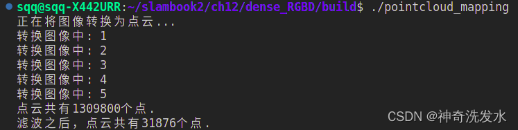
cout << "正在将图像转换为点云..." << endl;
// 定义点云使用的格式:这里用的是XYZRGB
typedef pcl::PointXYZRGB PointT;
//声明点云对象指针(点云类型为XYZ点云结构),并初始化该对象,pointcloud是一个泛型类,所以每次使用的记得申明
typedef pcl::PointCloud<PointT> PointCloud;
//将每张图片的像素,进行计算,转化为世界坐标系,并且在点云图中绘制
// 使用智能指针,创建一个空点云。这种指针用完会自动释放。
PointCloud::Ptr pointCloud(new PointCloud);
for (int i = 0; i < 5; i++)
{
PointCloud::Ptr current(new PointCloud);
cout << "转换图像中: " << i + 1 << endl;
cv::Mat color = colorImgs[i];
cv::Mat depth = depthImgs[i];
Eigen::Isometry3d T = poses[i];
for (int v = 0; v < color.rows; v++)
for (int u = 0; u < color.cols; u++)
{
unsigned int d = depth.ptr<unsigned short>(v)[u]; // 深度值
if (d == 0)
continue; // 为0表示没有测量到,跳过
//d存在值就加入点云
// 计算这个点的空间坐标
Eigen::Vector3d point;
point[2] = double(d) / depthScale;
point[0] = (u - cx) * point[2] / fx;
point[1] = (v - cy) * point[2] / fy;
Eigen::Vector3d pointWorld = T * point;
// 从rgb图像中获取它的颜色
// rgb是三通道的BGR格式图,所以按下面的顺序获取颜色
PointT p;// p的前三维存储坐标信息,后三位存储rgb颜色信息
p.x = pointWorld[0];
p.y = pointWorld[1];
p.z = pointWorld[2];
p.b = color.data[v * color.step + u * color.channels()];
p.g = color.data[v * color.step + u * color.channels() + 1];
p.r = color.data[v * color.step + u * color.channels() + 2];
current->points.push_back(p); // 把p加入到点云中
}
// depth filter and statistical removal
PointCloud::Ptr tmp(new PointCloud); //要滤波的对象是pointcloud,滤波的结果放到tmp中
//类StatisticalOutlierRemoval实现删除离群点的简单的滤波功能,如果一个点在给定搜索半径范围内邻近点数量小于给定阈值K,则判定为离群点并删除。
pcl::StatisticalOutlierRemoval<PointT> statistical_filter; // 外点去除滤波器
statistical_filter.setMeanK(50); // 设置在进行统计时考虑查询点邻近点数
statistical_filter.setStddevMulThresh(1.0); // 设置判断是否为离群点的阈值 。
statistical_filter.setInputCloud(current); // 设置待滤波的点云
statistical_filter.filter(*tmp); // 执行滤波处理,存储输出
(*pointCloud) += *tmp;
}
pointCloud->is_dense = false;
cout << "点云共有" << pointCloud->size() << "个点." << endl;
// voxel filter 降采样滤波器
pcl::VoxelGrid<PointT> voxel_filter;
double resolution = 0.03; //设置体素栅格叶大小
voxel_filter.setLeafSize(resolution, resolution, resolution); // 分别设置体素在XYZ方向上的尺寸
PointCloud::Ptr tmp(new PointCloud); // 设置需要过滤的点云给滤波对象
voxel_filter.setInputCloud(pointCloud);
voxel_filter.filter(*tmp); // 执行滤波处理,存储输出
tmp->swap(*pointCloud);
cout << "滤波之后,点云共有" << pointCloud->size() << "个点." << endl;
pcl::io::savePCDFileBinary("map.pcd", *pointCloud); //滤波结果保存
return 0;
}
运行结果

2.编译octomap
高仙
点云地图明显的缺陷:
1)点云地图通常规模很大,所以得到的pcd文件也会很大,需要大量的存储空间。然而这种“大”并不是必须的,它存储了很多不必要的细节。由于这些空间的占用,除非降低分辨率(降低分辨率又会导致地图质量下降),否则在有限的内存中,无法建模较大规模的环境。
2)点云地图无法处理运动物体。因为在生成点云地图时,我们只有“添加点”,而没有“当点消除时把它移除”的做法。但是生命在于运动,现实中,运动的物体又普遍存在,这使得点云地图不怎么实用。(考虑:能不能在点云地图中实现当点消除时把它移除,当地图规模不怎么大时就是用点云地图呢???毕竟点云地图的思路比较简单嘛)
所以现在我们来考虑一种灵活的、压缩的、又能随时更新的地图形式——八叉树(Octo-tree)
把一个大的三维空间细分为许多个小方块(或体素)(即从最大空间细分到最小空间的过程),就是一棵八叉树。
我们在建模点云地图时,利用了体素滤波器,限制了一个体素中只有一个点,但是点云仍然要比八叉树占用更多的空间,是因为:在八叉树中,我们在节点中存储它是否被占用的信息,当某个方块的所有子节点都被占局或都不被占据时,就不会展开这个节点(注意此处与点云的区别)。大多数的八叉树节点都无需展开到叶子层面。
octomap下载
octomap的代码主要含两个模块:本身的octomap和可视化工具octovis。octovis依赖于qt4和qglviewer
sudo apt-get install liboctomap-dev octovis
cmake
  mkdir build
  cd build
  cmake ..
  make
octomap的代码主要含两个模块:本身的octomap和可视化工具octovis。octovis依赖于qt4和qglviewer
sudo apt-get install libqt4-dev qt4-qmake libqglviewer-dev
查看
octovis octomap.bt
由于八叉树的原因,它的地图像是很多个小方块组成的(很像minecraft)。当分辨率较高时,方块很小;分辨率较低时,方块很大。每个方块表示该格被占据的概率。因此你可以查询某个方块或点“是否可以通过”,从而实现不同层次的导航。简而言之,环境较大时采用较低分辨率,而较精细的导航可采用较高分辨率.
每个小方块都有一个数描述它是否被占据。在最简单的情况下,可以用0-1两个数表示(太简单了所以没什么用)。通常还是用0~1之间的浮点数表示它被占据的概率。0.5表示未确定,越大则表示被占据的可能性越高,反之亦然
八叉树中的父亲节点占据概率,可以根据孩子节点的数值进行计算。比较简单的是取平均值或最大值。如果把八叉树按照占据概率进行渲染,不确定的方块渲染成透明的,确定占据的渲染成不透明的,就能看到我们平时见到的那种东西啦!
代码
#include <iostream>
#include <fstream>

using namespace std;

#include <opencv2/core/core.hpp>
#include <opencv2/highgui/highgui.hpp>

#include <octomap/octomap.h>    // for octomap

#include <eigen3/Eigen/Geometry>
#include <boost/format.hpp>  // for formating strings

int main(int argc, char **argv) {
    vector<cv::Mat> colorImgs, depthImgs;    // 彩色图和深度图
    vector<Eigen::Isometry3d> poses;         // 相机位姿

    ifstream fin("./data/pose.txt");
    if (!fin) {
        cerr << "cannot find pose file" << endl;
        return 1;
    }

    for (int i = 0; i < 5; i++) {
        boost::format fmt("./data/%s/%d.%s"); //图像文件格式
        colorImgs.push_back(cv::imread((fmt % "color" % (i + 1) % "png").str()));
        depthImgs.push_back(cv::imread((fmt % "depth" % (i + 1) % "png").str(), -1)); // 使用-1读取原始图像

        double data[7] = {0};
        for (int i = 0; i < 7; i++) {
            fin >> data[i];
        }
        Eigen::Quaterniond q(data[6], data[3], data[4], data[5]);
        Eigen::Isometry3d T(q);
        T.pretranslate(Eigen::Vector3d(data[0], data[1], data[2]));
        poses.push_back(T);
    }

    // 计算点云并拼接
    // 相机内参
    double cx = 319.5;
    double cy = 239.5;
    double fx = 481.2;
    double fy = -480.0;
    double depthScale = 5000.0;

    cout << "正在将图像转换为 Octomap ..." << endl;

    // octomap tree创建八叉树
    octomap::OcTree tree(0.01); // 参数为分辨率

    for (int i = 0; i < 5; i++) {
        cout << "转换图像中: " << i + 1 << endl;
        cv::Mat color = colorImgs[i];
        cv::Mat depth = depthImgs[i];
        Eigen::Isometry3d T = poses[i];

        octomap::Pointcloud cloud;  // the point cloud in octomap octomap中的点云

        for (int v = 0; v < color.rows; v++)
            for (int u = 0; u < color.cols; u++) {
                unsigned int d = depth.ptr<unsigned short>(v)[u]; // 深度值
                if (d == 0) continue; // 为0表示没有测量到
                Eigen::Vector3d point;
                point[2] = double(d) / depthScale;
                point[0] = (u - cx) * point[2] / fx;
                point[1] = (v - cy) * point[2] / fy;
                Eigen::Vector3d pointWorld = T * point;//相机->世界
                // 将世界坐标系的点放入点云
                cloud.push_back(pointWorld[0], pointWorld[1], pointWorld[2]);
            }

        // 将点云存入八叉树地图,给定原点,这样可以计算投射线
        tree.insertPointCloud(cloud, octomap::point3d(T(0, 3), T(1, 3), T(2, 3)));
    }

    // 更新中间节点的占据信息并写入磁盘
    tree.updateInnerOccupancy();//更新中间节点的占据信息并写入磁盘
    cout << "saving octomap ... " << endl;
    tree.writeBinary("octomap.bt"); //将八叉树地图写入二进制文件
    return 0;
}
运行结果
octomap里的pointcloud是一种射线的形式,只有末端才存在被占据的点,中途的点则是没被占据的。这会使一些重叠地方处理的更好。

3.surfel_mapping.cpp
参考

点云网格化就是用点云生成网格,最后得到的是一个连续(相对于前面的离散点)的表面。如果再加上纹理贴图,就能得到和真实物体一样的三维模型
贪婪投影三角化算法参考
参考2
将三维点通过法线投影到某一平面,然后对投影得到的点云作平面内的三角化,从而得到各点的连接关系。在平面区域三角化的过程中用到了基于 Delaunay 的 空间区域增长算法,该方法通过选取一个样本三角片作为初始曲面,不断扩张曲面边界,最后形成一张完整的三角网格曲面。最后根据投影点云的连接关系确定各原始三维点间的拓扑连接,所得三角格网即为重建得到的曲面模型。
具体方法是先将有向点云投影到某一局部二维坐标平面内,再在坐标平面内进行平面内的三角化,再根据平面内三位点的拓扑连接关系获得一个三角网格曲面模型
网格
四角网格和三角网格
 顶点:每个三角形都有三个顶点,各顶点都有可能和其他三角形共享。
边:连接两个顶点的边,每个三角形有三条边。
面:每个三角形对应一个面,我们可以用顶点或边列表表示面。
点云进行网格生成一般分为两大类方法:
1、插值法。顾名思义,也就是重建的曲面都是通过原始的数据点得到的
2、逼近法。用分片线性曲面或其他曲面来逼近原始数据点,得到的重建曲面是原始点集的一个逼近。
点云贪心三角化原理
   `Delaunay三角剖分`
   定义:假设点集中的一条边e(两个端点为a,b),e若满足下列条件,则称之为Delaunay边:存在一个圆经过a,b两点,圆内(圆上最多三点共圆)不含点集中任何其他的点。而Delaunay三角化就是指三角网格均是由Delaunay边组成,并满足`最小角最大原则`(在点集可能形成的三角剖分中,Delaunay三角剖分所形成的三角形的最小角最大)。
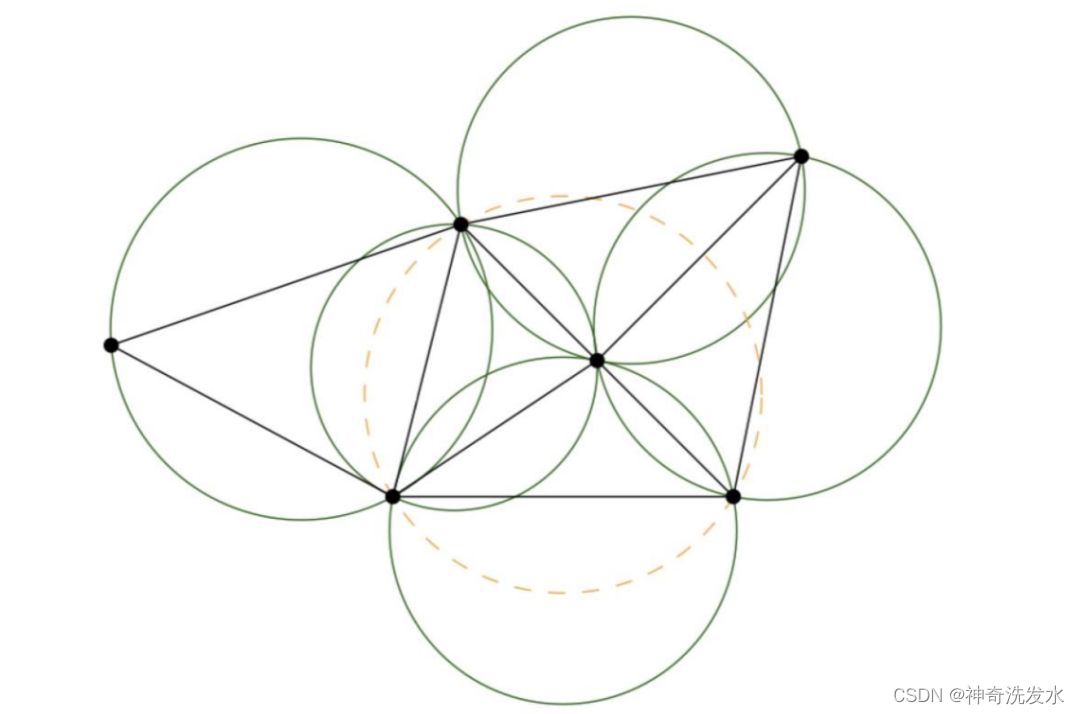 所有三角形的顶点是不是都不在其他三角形的外接圆内
简便判断方法:观察具有公共边缘BD的两个三角形ABD和BCD,如果角度α和γ之和小于或等于180°,则三角形满足Delaunay条件。按照这个标准下图左、中都不满足Delaunay条件,只有右图满足。
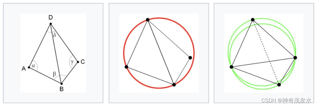
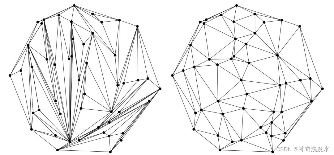 左侧不是,右侧是
PCL中采用将三维点云投影到二维平面的方法来实现三角剖分, 具体采用贪婪三角化算法。
其过程为:
1:计算点云中点的法线,再将点云通过法线投影到二维坐标平面。
2:使用基于Delaunay三角剖分的空间区域增长算法完成平面点集的三角化。
3:根据投影点云的连接关系确定原始三维点云间的拓扑关系,最终得到曲面模型。
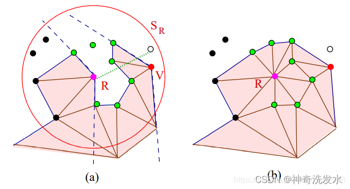
算法流程:
1.Kd-tree最近邻搜索:给定参考点 P ,在半径为 r 的球内搜索该点的最近k-领域来创建点p的领域。 $ r=\mu d_0 $,其中 d 0 是点 p和最近相邻点的距离; $ \mu $是用户考虑点云密度的自定义常数。
使用切平面的进行领域投影:将第一步找出来的点集 $ C_r§ $,通过点
P
P
P的法向量投影到一个平面上,该平面与领域形成的表面大致相切,并按角度排序。
修剪pruning:通过可见性和距离等标准,删除$C_r§ $中的某些点。依次连接到点 P,以及前后连接,形成满足(1)具有最大角度标准和(2)最小角度标准(可选的)的三角形。点云修剪一般会依赖于很多标准。
a. 按距离修剪:使用kd-tree搜索候选邻近点,排除距离特别远的点;
b. 进一步排除:位于参考点为中心的球 $S_R $之外的其他点是不能作为候选点。
c. 投影:应用距离标准获得的选点集投影到近似切平面;
d. 角度排序:以参考点为原点定义新的局部坐标系,前一步的投影平面作为xy平面;候选点集中的所有点都投影到这个平面。候选点的角度 $ \theta θ $为局部坐标系的x轴与从原点 P P P到投影的候选点的向量的夹角;并将候选点按照角度排序。
f. 可见性准则:丢弃可能形成自相交网格的点。
算法定义了两种边缘类型来检查这种情况:
(1) 边界边:仅有一个相邻三角形的边,这些边连接“边缘”点或者“边界”点;
(2) 内部边:连接“完成”点与其他任何点。下图展示了 R点的可见性测试。所有黑色的点都在 R R R的边界边之外;白色的点则被其他边遮挡;而点 V 则是因为 R 点在它的边界边之外。
MLS
参考
用MLS表面重建法平滑点云
课程介绍了使用MLS (Moving Least Squares,移动最小二乘)表面重建法平滑和重采样噪声数据。一些距离测量误差导致的点云不规则很难用统计分析方法去除。当没法获得额外数据,可以采用重采样算法(通过对周围数据点进行高阶多项式内插)来重建表面缺失部分。通过重采样,可以纠正小误差,配准误差导致的“double walls” (重影)现象可减轻。因为表面被平滑,估计的法向量和曲率也更加平滑。
为了近若干近邻点的表面,使用定义在参考平面上的二元多项式高度函数(bivariate polynomial height function)。
参考
inline void setComputeNormals(bool compute_normals) 我们都知道表面重构时需要估计点云的法向量,这里MLS提供了一种方法来估计点云法向量。(如果是true的话注意输出数据格式)。
inline void setComputeNormals(bool compute_normals) 我们都知道表面重构时需要估计点云的法向量,这里MLS提供了一种方法来估计点云法向量。(如果是true的话注意输出数据格式)。
inline void setSearchMethod(const KdTreePtr&tree) 使用kdTree加速搜索
inline void setPolynomialOrder(int order) MLS拟合曲线的阶数,这个阶数在构造函数里默认是2,但是参考文献给出最好选择3或者4,当然不难得出随着阶数的增加程序运行的时间也增加。
inline voidsetPolynomailFit(bool polynomial_fit) 对于法线的估计是有多项式还是仅仅依靠切线。
inline void setSearchRadius(double radius) 确定搜索的半径。也就是说在这个半径里进行表面映射和曲面拟合。从实验结果可知:半径越小拟合后曲面的失真度越小,反之有可能出现过拟合的现象。
KDTree
参考
其实KDTree就是二叉查找树(Binary Search Tree,BST)的变种。二叉查找树的性质如下:
1)若它的左子树不为空,则左子树上所有结点的值均小于它的根结点的值;
2)若它的右子树不为空,则右子树上所有结点的值均大于它的根结点的值;
3)它的左、右子树也分别为二叉排序树;
例如:
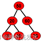
kd-tree,是k维的二叉树。其中的每一个节点都是k维的数据,数据结构如下所示
struct kdtree{
    Node-data - 数据矢量   数据集中某个数据点,是n维矢量(这里也就是k维)
    Range     - 空间矢量   该节点所代表的空间范围
    split     - 整数       垂直于分割超平面的方向轴序号
    Left      - kd树       由位于该节点分割超平面左子空间内所有数据点所构成的k-d树
    Right     - kd树       由位于该节点分割超平面右子空间内所有数据点所构成的k-d树
    parent    - kd树       父节点
}
代码:
//
// Created by gaoxiang on 19-4-25.
//
#include <pcl/point_cloud.h>
#include <pcl/point_types.h>
#include <pcl/io/pcd_io.h>
#include <pcl/visualization/pcl_visualizer.h>
//PCLVisualizer是PCL中全功能的可视化类。虽然在使用上比CloudViewer更加复杂,
//但是它功能更加强大,提供了比如显示法线、绘制图形以及多视点等特性。
#include <pcl/kdtree/kdtree_flann.h>//kdtree类定义头文件,kd-tree的维度是3
#include <pcl/surface/surfel_smoothing.h>
#include <pcl/surface/mls.h>//移动最小二乘法
#include <pcl/surface/gp3.h>
#include <pcl/surface/impl/mls.hpp>
// typedefs
typedef pcl::PointXYZRGB PointT;//定义点的类型 XYZ,RGB
typedef pcl::PointCloud<PointT> PointCloud;//定义点云
typedef pcl::PointCloud<PointT>::Ptr PointCloudPtr;//定义点云指针
typedef pcl::PointXYZRGBNormal SurfelT;//网格数据类型 XYZ,RGB,强度曲率
//PointXYZRGBNormal{
// PCL_ADD_POINT4D;//xyz实际坐标或者xyz1齐次做标
// PCL_ADD_NORMAL4D;//bgr颜色
// union
// {
// struct
// {
// float intensity;//强度
// float curvature;//曲率
// };
// float data_c[4];
// };
//}
typedef pcl::PointCloud<SurfelT> SurfelCloud;//曲率的点云
typedef pcl::PointCloud<SurfelT>::Ptr SurfelCloudPtr;//曲率的点云指针
SurfelCloudPtr reconstructSurface(
const PointCloudPtr &input, float radius, int polynomial_order) {
pcl::MovingLeastSquares<PointT, SurfelT> mls;
pcl::search::KdTree<PointT>::Ptr tree(new pcl::search::KdTree<PointT>);
// struct kdtree{
// Node-data - 数据矢量 数据集中某个数据点,是n维矢量(这里也就是k维)
// Range - 空间矢量 该节点所代表的空间范围
// split - 整数 垂直于分割超平面的方向轴序号
// Left - kd树 由位于该节点分割超平面左子空间内所有数据点所构成的k-d树
// Right - kd树 由位于该节点分割超平面右子空间内所有数据点所构成的k-d树
// parent - kd树 父节点
// }
//最小二乘法(MLS)点云平滑参数设置
//此类并不能输出拟合后的表面,不能生成Mesh或者Triangulations,只是将点云进行了MLS的映射,使得输出的点云更加平滑
mls.setSearchMethod(tree); //设置查找方法
mls.setSearchRadius(radius);//设置球面查找半径,半径以内全部为临近点
//在这个半径里进行表面映射和曲面拟合。从实验结果可知:半径越小拟合后曲面的失真度越小,反之有可能出现过拟合的现象
mls.setComputeNormals(true);//设置计算法向量,当法线估计标志位设置为true时,输出向量必须加上
mls.setSqrGaussParam(radius * radius);//设置高斯函数,用作权重
mls.setPolynomialFit(polynomial_order > 1);//使用多项式拟合曲面和法向量的条件,如果满足条件设为1,有多项式或仅切线。
mls.setPolynomialOrder(polynomial_order);//设置拟合多项式的次数
mls.setInputCloud(input);//输入点云
SurfelCloudPtr output(new SurfelCloud);
// 曲面重建
mls.process(*output);//输出结果
return (output);
}
pcl::PolygonMeshPtr triangulateMesh(const SurfelCloudPtr &surfels) {
// Create search tree*
pcl::search::KdTree<SurfelT>::Ptr tree(new pcl::search::KdTree<SurfelT>);
tree->setInputCloud(surfels);//输入数据
// Initialize objects初始化目标
pcl::GreedyProjectionTriangulation<SurfelT> gp3;//3角贪心算法 定义三角化对象
pcl::PolygonMeshPtr triangles(new pcl::PolygonMesh);//创建指针,存储最终三角化的网络模型
// Set the maximum distance between connected points (maximum edge length)设置相邻点的最大距离
gp3.setSearchRadius(0.05);//设置球面半径,KNN的球半径,在3角化的k最邻点使用
// Set typical values for the parameters
gp3.setMu(2.5);//设置每个点的最终搜索半径的倍数,典型值(2.5-3),这样使得算法自适应点云密度的变化
gp3.setMaximumNearestNeighbors(100);//设置样本点最多可搜索的邻域个数,典型值是50-100
//setMaximumSurfaceAgle和setNormalConsistency 用于处理有尖锐边缘或棱角的情况,以及表面的两面非常接近的情况。
gp3.setMaximumSurfaceAngle(M_PI / 4); // 设置某点法线方向偏离样本点法线的最大角度45°,如果超过,连接时不考虑该点
gp3.setMinimumAngle(M_PI / 18); // 设置三角化后得到的三角形内角的最小的角度为10°
gp3.setMaximumAngle(2 * M_PI / 3); // 设置三角化后得到的三角形内角的最大角度为120°
gp3.setNormalConsistency(true);//设置该参数为true保证法线朝向一致,设置为false的话不会进行法线一致性检查
// Get result得到结果
gp3.setInputCloud(surfels);//设置输入点云为有向点云
gp3.setSearchMethod(tree);//输入查找树,设置输入方式
gp3.reconstruct(*triangles);//得到重建后的网格
return triangles;
}
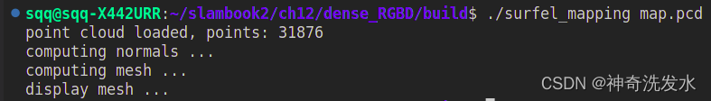
int main(int argc, char **argv) {
// Load the points
PointCloudPtr cloud(new PointCloud);//加载点云
if (argc == 0 || pcl::io::loadPCDFile(argv[1], *cloud)) {//读取项目路径下的pcd点云
cout << "failed to load point cloud!";
return 1;
}
cout << "point cloud loaded, points: " << cloud->points.size() << endl;
// Compute surface elements
cout << "computing normals ... " << endl;
double mls_radius = 0.05, polynomial_order = 2;
auto surfels = reconstructSurface(cloud, mls_radius, polynomial_order);
// Compute a greedy surface triangulation
cout << "computing mesh ... " << endl;
pcl::PolygonMeshPtr mesh = triangulateMesh(surfels);
cout << "display mesh ... " << endl;
pcl::visualization::PCLVisualizer vis;
vis.addPolylineFromPolygonMesh(*mesh, "mesh frame");
vis.addPolygonMesh(*mesh, "mesh");
vis.resetCamera();
vis.spin();//.开启永久循环暂留
}
etMaximumSurfaceAgle和setNormalConsistency 其实是用于处理有尖锐边缘或棱角的情况,以及表面的两面非常接近的情况。比如setMaximumSurfaceAgle,表示如果某点的法线偏离了参考点超过了指定的角度(典型为45°),那么它们就不会与当前点连接。
setNormalConsistency 的话,注释里也说了,是保证法线朝向一致。因为大多数表面法线估计方法得到的法线,即使是在锐利的边缘之间也是平滑的过渡。因为不是所有的法线估计方法都能保证法线的方向一致。通常情况下,设置为false对大多数数据集有效。
spin()函数画面永久停留
spinOnce(1,false)函数给定时间内循环
void spinOnce(int time = 1, bool force_redraw = false);
运行结果
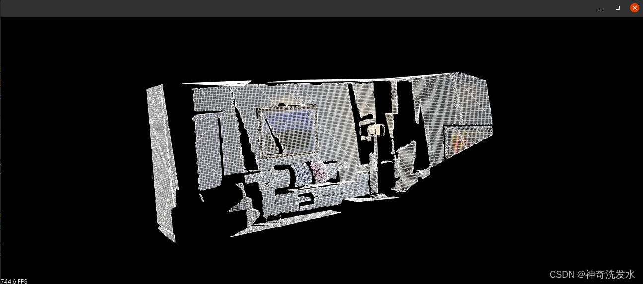 改了下半径0.01


cmakelists.txt
cmake_minimum_required(VERSION 2.8)

set(CMAKE_BUILD_TYPE Release)
set(CMAKE_CXX_FLAGS "-std=c++14 -O2")

# opencv
find_package(OpenCV REQUIRED)
include_directories(${OpenCV_INCLUDE_DIRS})

# eigen
include_directories("/usr/include/eigen3/")

# pcl
find_package(PCL REQUIRED)
include_directories(${PCL_INCLUDE_DIRS})
add_definitions(${PCL_DEFINITIONS})

# octomap
find_package(octomap REQUIRED)
include_directories(${OCTOMAP_INCLUDE_DIRS})

add_executable(pointcloud_mapping pointcloud_mapping.cpp)
target_link_libraries(pointcloud_mapping ${OpenCV_LIBS} ${PCL_LIBRARIES})

add_executable(octomap_mapping octomap_mapping.cpp)
target_link_libraries(octomap_mapping ${OpenCV_LIBS} ${PCL_LIBRARIES} ${OCTOMAP_LIBRARIES} fmt)

add_executable(surfel_mapping surfel_mapping.cpp)
target_link_libraries(surfel_mapping ${OpenCV_LIBS} ${PCL_LIBRARIES} fmt)


 2144
2144


 被折叠的 条评论
为什么被折叠?
被折叠的 条评论
为什么被折叠?
 到【灌水乐园】发言


