SLAM第12讲 建图实践部分

1 实践：单目稠密重建

1.1 我们需要下载示例程序所需要的数据集http://rpg.ifi.uzh.ch/datasets/remode_test_data.zip。它提供了一架无人机采集到的单目俯视图像，共200张，同时提供了每张图像对应的位姿。下面我们通过这些数据估算第一帧图像每个像素对应的深度值，即进行单目稠密重建。

估计稠密深度的步骤：

• 假设所有像素的深度满足某个初始的高斯分布；
• 当新数据产生时，通过极线搜索和块匹配确定投影点位置；
• 根据几何关系计算三角化后的深度及不确定性；
• 将当前观测融合进上一次的估计中。若收敛则停止计算，否则返回第二步；

这里所说的深度值是相机光心到空间路标点的长度，而不是针孔相机模型中的像素点的z值。
主程序：

int main(int argc, char **argv) {
    if (argc != 2) {
        cout << "Usage: dense_mapping path_to_test_dataset" << endl;
        return -1;
    }

    // 从数据集读取数据
    vector<string> color_image_files;
    vector<SE3d> poses_TWC;
    Mat ref_depth;
    bool ret = readDatasetFiles(argv[1], color_image_files, poses_TWC, ref_depth);
    if (ret == false) {
        cout << "Reading image files failed!" << endl;
        return -1;
    }
    cout << "read total " << color_image_files.size() << " files." << endl;

    // 第一张图
    Mat ref = imread(color_image_files[0], 0);                // gray-scale image
    SE3d pose_ref_TWC = poses_TWC[0];
    double init_depth = 3.0;    // 深度初始值
    double init_cov2 = 3.0;     // 方差初始值
    Mat depth(height, width, CV_64F, init_depth);             // 深度图
    Mat depth_cov2(height, width, CV_64F, init_cov2);         // 深度图方差

    for (int index = 1; index < color_image_files.size(); index++) {
        cout << "*** loop " << index << " ***" << endl;
        Mat curr = imread(color_image_files[index], 0);
        if (curr.data == nullptr) continue;
        SE3d pose_curr_TWC = poses_TWC[index];
        SE3d pose_T_C_R = pose_curr_TWC.inverse() * pose_ref_TWC;   // 坐标转换关系： T_C_W * T_W_R = T_C_R
        update(ref, curr, pose_T_C_R, depth, depth_cov2);
        evaludateDepth(ref_depth, depth);
        plotDepth(ref_depth, depth);
        imshow("image", curr);
        waitKey(1);
    }

    cout << "estimation returns, saving depth map ..." << endl;
    imwrite("depth.png", depth);
    cout << "done." << endl;

    return 0;
}

从主程序剖析程序的处理流程：
1> 定义了readDatesetFiles(）函数利用创建的fin文件流对象从对应的数据集路径下去获取200帧图像的名称以及所对应的相机的位姿，无需重新去打开文件读取图片名称，位姿文件每行的开头就是对应的200张图片的名称，然后去获取第一幅图像的所有像素点的深度信息。

bool readDatasetFiles(
    const string &path,
    vector<string> &color_image_files,
    std::vector<SE3d> &poses,
    cv::Mat &ref_depth) {
    ifstream fin(path + "/first_200_frames_traj_over_table_input_sequence.txt");
    if (!fin) return false;

    while (!fin.eof()) {
        // 数据格式：图像文件名 tx, ty, tz, qx, qy, qz, qw ，注意是 TWC 而非 TCW
        string image;
        fin >> image;
        double data[7];
        for (double &d:data) fin >> d;

        color_image_files.push_back(path + string("/images/") + image);
        poses.push_back(
            SE3d(Quaterniond(data[6], data[3], data[4], data[5]),
                 Vector3d(data[0], data[1], data[2]))
        );
        if (!fin.good()) break;
    }
    fin.close();

    // load reference depth
    fin.open(path + "/depthmaps/scene_000.depth");
    ref_depth = cv::Mat(height, width, CV_64F);
    if (!fin) return false;
    for (int y = 0; y < height; y++)
        for (int x = 0; x < width; x++) {
            double depth = 0;
            fin >> depth;
            ref_depth.ptr<double>(y)[x] = depth / 100.0;
        }

    return true;
}

2> 获取完数据集中的内容后，紧接着对第一幅图初始化深度图和深度图方差

double init_depth = 3.0;    // 深度初始值
 double init_cov2 = 3.0;     // 方差初始值
 Mat depth(height, width, CV_64F, init_depth);             // 深度图
 Mat depth_cov2(height, width, CV_64F, init_cov2);         // 深度图方差

3> 第一帧图像与剩下的其他图像的相机位姿的变换关系：

SE3d pose_curr_TWC = poses_TWC[index];
 SE3d pose_T_C_R = pose_curr_TWC.inverse() * pose_ref_TWC;   // 坐标转换关系： T_C_W * T_W_R = T_C_R

4> 对深度图和深度方差进行更新update(ref, curr, pose_T_C_R, depth, depth_cov2);

// 对整个深度图进行更新
bool update(const Mat &ref, const Mat &curr, const SE3d &T_C_R, Mat &depth, Mat &depth_cov2) {
    for (int x = boarder; x < width - boarder; x++)
        for (int y = boarder; y < height - boarder; y++) {
            // 遍历每个像素
            if (depth_cov2.ptr<double>(y)[x] < min_cov || depth_cov2.ptr<double>(y)[x] > max_cov) // 深度已收敛或发散
                continue;
            // 在极线上搜索 (x,y) 的匹配
            Vector2d pt_curr;
            Vector2d epipolar_direction;
            bool ret = epipolarSearch(
                ref,
                curr,
                T_C_R,
                Vector2d(x, y),
                depth.ptr<double>(y)[x],
                sqrt(depth_cov2.ptr<double>(y)[x]),
                pt_curr,
                epipolar_direction
            );

            if (ret == false) // 匹配失败
                continue;

            // 取消该注释以显示匹配
            // showEpipolarMatch(ref, curr, Vector2d(x, y), pt_curr);

            // 匹配成功，更新深度图
            updateDepthFilter(Vector2d(x, y), pt_curr, T_C_R, epipolar_direction, depth, depth_cov2);
        }
}

设定深度图方差的阈值，小与min_cov我们认为对应像素的深度已收敛，若大与max_cov则发散，然后在极线段上去匹配对应的像素点，通过三角化来取定确定深度进而优化像素的深度。使用epipolarSearch() 进行极线搜索。根据获取到的第一幅图像的深度信息把像素点从像素坐标转到相机坐标下Vector3d f_ref = px2cam(pt_ref);,然后对其极每个点的坐标进行归一化，使其都在相机的归一化平面坐标系下，f_ref.normalize(); 该像素点对应的空间点的初始化坐标为Vector3d P_ref = f_ref * depth_mu; // 参考帧的 P 向量 ,然后将像素空间点通过前面算出的T_C_R将其转换到第二帧图像所对应的相机的坐标系下通过Vector2d px_mean_curr = cam2px(T_C_R * P_ref); // 按深度均值投影的像素将其转为当前图像下的像素坐标。“空间点到光心的直线上所有点都在同一极线上”，因此我们取两个不同深度值（以均值为中心左右各取3倍标准差为半径，取最大值和最小值）做重投影，两点确定一条直线，也就得到了极线段

double d_min = depth_mu - 3 * depth_cov, d_max = depth_mu + 3 * depth_cov;
if (d_min < 0.1) d_min = 0.1;
Vector2d px_min_curr = cam2px(T_C_R * (f_ref * d_min));    // 按最小深度投影的像素
Vector2d px_max_curr = cam2px(T_C_R * (f_ref * d_max));    // 按最大深度投影的像素
 Vector2d epipolar_line = px_max_curr - px_min_curr;    // 极线（线段形式）
 epipolar_direction = epipolar_line;        // 极线方向

然后将极线的归一化，以深度均值为中心，左右取半长度，步长为sqrt(2 * best_ncc)来找匹配点，px_mean_curr是带有深度方差的投影点，在极线上得到一个沿着NCC分布的确定匹配点px_curr，匹配好后
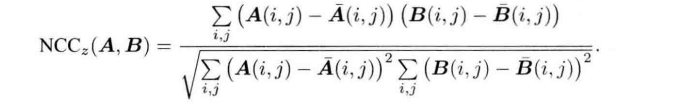
计算匹配点与参考点的NCC值

double NCC(
    const Mat &ref, const Mat &curr,
    const Vector2d &pt_ref, const Vector2d &pt_curr) {
    // 零均值-归一化互相关
    // 先算均值
    double mean_ref = 0, mean_curr = 0;
    vector<double> values_ref, values_curr; // 参考帧和当前帧的均值
    for (int x = -ncc_window_size; x <= ncc_window_size; x++)
        for (int y = -ncc_window_size; y <= ncc_window_size; y++) {
            double value_ref = double(ref.ptr<uchar>(int(y + pt_ref(1, 0)))[int(x + pt_ref(0, 0))]) / 255.0;
            mean_ref += value_ref;

            double value_curr = getBilinearInterpolatedValue(curr, pt_curr + Vector2d(x, y));
            mean_curr += value_curr;

            values_ref.push_back(value_ref);
            values_curr.push_back(value_curr);
        }

    mean_ref /= ncc_area;
    mean_curr /= ncc_area;

    // 计算 Zero mean NCC
    double numerator = 0, demoniator1 = 0, demoniator2 = 0;
    for (int i = 0; i < values_ref.size(); i++) {
        double n = (values_ref[i] - mean_ref) * (values_curr[i] - mean_curr);
        numerator += n;
        demoniator1 += (values_ref[i] - mean_ref) * (values_ref[i] - mean_ref);
        demoniator2 += (values_curr[i] - mean_curr) * (values_curr[i] - mean_curr);
    }
    return numerator / sqrt(demoniator1 * demoniator2 + 1e-10);   // 防止分母出现零
}

// 双线性灰度插值
inline double getBilinearInterpolatedValue(const Mat &img, const Vector2d &pt) {
    uchar *d = &img.data[int(pt(1, 0)) * img.step + int(pt(0, 0))];
    double xx = pt(0, 0) - floor(pt(0, 0));
    double yy = pt(1, 0) - floor(pt(1, 0));
    return ((1 - xx) * (1 - yy) * double(d[0]) +
            xx * (1 - yy) * double(d[1]) +
            (1 - xx) * yy * double(d[img.step]) +
            xx * yy * double(d[img.step + 1])) / 255.0;
}

最后当图像中的像素点匹配完成后，进行深度图的更新

bool updateDepthFilter(
    const Vector2d &pt_ref,
    const Vector2d &pt_curr,
    const SE3d &T_C_R,
    const Vector2d &epipolar_direction,
    Mat &depth,
    Mat &depth_cov2) {
    // 用三角化计算深度
    SE3d T_R_C = T_C_R.inverse();
    Vector3d f_ref = px2cam(pt_ref);
    f_ref.normalize();
    Vector3d f_curr = px2cam(pt_curr);
    f_curr.normalize();

    // 方程
    // d_ref * f_ref = d_cur * ( R_RC * f_cur ) + t_RC
    // f2 = R_RC * f_cur
    // 转化成下面这个矩阵方程组
    // => [ f_ref^T f_ref, -f_ref^T f2 ] [d_ref]   [f_ref^T t]
    //    [ f_cur^T f_ref, -f2^T f2    ] [d_cur] = [f2^T t   ]
    Vector3d t = T_R_C.translation();
    Vector3d f2 = T_R_C.so3() * f_curr;
    Vector2d b = Vector2d(t.dot(f_ref), t.dot(f2));
    Matrix2d A;
    A(0, 0) = f_ref.dot(f_ref);
    A(0, 1) = -f_ref.dot(f2);
    A(1, 0) = -A(0, 1);
    A(1, 1) = -f2.dot(f2);
    Vector2d ans = A.inverse() * b;
    Vector3d xm = ans[0] * f_ref;           // ref 侧的结果
    Vector3d xn = t + ans[1] * f2;          // cur 结果
    Vector3d p_esti = (xm + xn) / 2.0;      // P的位置，取两者的平均
    double depth_estimation = p_esti.norm();   // 深度值

    // 计算不确定性（以一个像素为误差）
    Vector3d p = f_ref * depth_estimation;
    Vector3d a = p - t;
    double t_norm = t.norm();
    double a_norm = a.norm();
    double alpha = acos(f_ref.dot(t) / t_norm);
    double beta = acos(-a.dot(t) / (a_norm * t_norm));
    Vector3d f_curr_prime = px2cam(pt_curr + epipolar_direction);
    f_curr_prime.normalize();
    double beta_prime = acos(f_curr_prime.dot(-t) / t_norm);
    double gamma = M_PI - alpha - beta_prime;
    double p_prime = t_norm * sin(beta_prime) / sin(gamma);
    double d_cov = p_prime - depth_estimation;
    double d_cov2 = d_cov * d_cov;

    // 高斯融合
    double mu = depth.ptr<double>(int(pt_ref(1, 0)))[int(pt_ref(0, 0))];
    double sigma2 = depth_cov2.ptr<double>(int(pt_ref(1, 0)))[int(pt_ref(0, 0))];

    double mu_fuse = (d_cov2 * mu + sigma2 * depth_estimation) / (sigma2 + d_cov2);
    double sigma_fuse2 = (sigma2 * d_cov2) / (sigma2 + d_cov2);

    depth.ptr<double>(int(pt_ref(1, 0)))[int(pt_ref(0, 0))] = mu_fuse;
    depth_cov2.ptr<double>(int(pt_ref(1, 0)))[int(pt_ref(0, 0))] = sigma_fuse2;

    return true;
}

最后更新先验信息：evaludateDepth(ref_depth, depth);

整个代码如下：

#include <iostream>
#include <vector>
#include <fstream>

using namespace std;

#include <boost/timer.hpp>

// for sophus
#include <sophus/se3.hpp>

using Sophus::SE3d;

// for eigen
#include <Eigen/Core>
#include <Eigen/Geometry>

using namespace Eigen;

#include <opencv2/core/core.hpp>
#include <opencv2/highgui/highgui.hpp>
#include <opencv2/imgproc/imgproc.hpp>

using namespace cv;

/**********************************************
* 本程序演示了单目相机在已知轨迹下的稠密深度估计
* 使用极线搜索 + NCC 匹配的方式，与书本的 12.2 节对应
* 请注意本程序并不完美，你完全可以改进它——我其实在故意暴露一些问题(这是借口)。
***********************************************/

// ------------------------------------------------------------------
// parameters
const int boarder = 20;         // 边缘宽度
const int width = 640;          // 图像宽度
const int height = 480;         // 图像高度
const double fx = 481.2f;       // 相机内参
const double fy = -480.0f;
const double cx = 319.5f;
const double cy = 239.5f;
const int ncc_window_size = 3;    // NCC 取的窗口半宽度
const int ncc_area = (2 * ncc_window_size + 1) * (2 * ncc_window_size + 1); // NCC窗口面积
const double min_cov = 0.1;     // 收敛判定：最小方差
const double max_cov = 10;      // 发散判定：最大方差

// ------------------------------------------------------------------
// 重要的函数
/// 从 REMODE 数据集读取数据
bool readDatasetFiles(
    const string &path,
    vector<string> &color_image_files,
    vector<SE3d> &poses,
    cv::Mat &ref_depth
);

/**
 * 根据新的图像更新深度估计
 * @param ref           参考图像
 * @param curr          当前图像
 * @param T_C_R         参考图像到当前图像的位姿
 * @param depth         深度
 * @param depth_cov     深度方差
 * @return              是否成功
 */
bool update(
    const Mat &ref,
    const Mat &curr,
    const SE3d &T_C_R,
    Mat &depth,
    Mat &depth_cov2
);

/**
 * 极线搜索
 * @param ref           参考图像
 * @param curr          当前图像
 * @param T_C_R         位姿
 * @param pt_ref        参考图像中点的位置
 * @param depth_mu      深度均值
 * @param depth_cov     深度方差
 * @param pt_curr       当前点
 * @param epipolar_direction  极线方向
 * @return              是否成功
 */
bool epipolarSearch(
    const Mat &ref,
    const Mat &curr,
    const SE3d &T_C_R,
    const Vector2d &pt_ref,
    const double &depth_mu,
    const double &depth_cov,
    Vector2d &pt_curr,
    Vector2d &epipolar_direction
);

/**
 * 更新深度滤波器
 * @param pt_ref    参考图像点
 * @param pt_curr   当前图像点
 * @param T_C_R     位姿
 * @param epipolar_direction 极线方向
 * @param depth     深度均值
 * @param depth_cov2    深度方向
 * @return          是否成功
 */
bool updateDepthFilter(
    const Vector2d &pt_ref,
    const Vector2d &pt_curr,
    const SE3d &T_C_R,
    const Vector2d &epipolar_direction,
    Mat &depth,
    Mat &depth_cov2
);

/**
 * 计算 NCC 评分
 * @param ref       参考图像
 * @param curr      当前图像
 * @param pt_ref    参考点
 * @param pt_curr   当前点
 * @return          NCC评分
 */
double NCC(const Mat &ref, const Mat &curr, const Vector2d &pt_ref, const Vector2d &pt_curr);

// 双线性灰度插值
inline double getBilinearInterpolatedValue(const Mat &img, const Vector2d &pt) {
    uchar *d = &img.data[int(pt(1, 0)) * img.step + int(pt(0, 0))];
    double xx = pt(0, 0) - floor(pt(0, 0));
    double yy = pt(1, 0) - floor(pt(1, 0));
    return ((1 - xx) * (1 - yy) * double(d[0]) +
            xx * (1 - yy) * double(d[1]) +
            (1 - xx) * yy * double(d[img.step]) +
            xx * yy * double(d[img.step + 1])) / 255.0;
}

// ------------------------------------------------------------------
// 一些小工具
// 显示估计的深度图
void plotDepth(const Mat &depth_truth, const Mat &depth_estimate);

// 像素到相机坐标系
inline Vector3d px2cam(const Vector2d px) {
    return Vector3d(
        (px(0, 0) - cx) / fx,
        (px(1, 0) - cy) / fy,
        1
    );
}

// 相机坐标系到像素
inline Vector2d cam2px(const Vector3d p_cam) {
    return Vector2d(
        p_cam(0, 0) * fx / p_cam(2, 0) + cx,
        p_cam(1, 0) * fy / p_cam(2, 0) + cy
    );
}

// 检测一个点是否在图像边框内
inline bool inside(const Vector2d &pt) {
    return pt(0, 0) >= boarder && pt(1, 0) >= boarder
           && pt(0, 0) + boarder < width && pt(1, 0) + boarder <= height;
}

// 显示极线匹配
void showEpipolarMatch(const Mat &ref, const Mat &curr, const Vector2d &px_ref, const Vector2d &px_curr);

// 显示极线
void showEpipolarLine(const Mat &ref, const Mat &curr, const Vector2d &px_ref, const Vector2d &px_min_curr,
                      const Vector2d &px_max_curr);

/// 评测深度估计
void evaludateDepth(const Mat &depth_truth, const Mat &depth_estimate);
// ------------------------------------------------------------------


int main(int argc, char **argv) {
    if (argc != 2) {
        cout << "Usage: dense_mapping path_to_test_dataset" << endl;
        return -1;
    }

    // 从数据集读取数据
    vector<string> color_image_files;
    vector<SE3d> poses_TWC;
    Mat ref_depth;
    bool ret = readDatasetFiles(argv[1], color_image_files, poses_TWC, ref_depth);
    if (ret == false) {
        cout << "Reading image files failed!" << endl;
        return -1;
    }
    cout << "read total " << color_image_files.size() << " files." << endl;

    // 第一张图
    Mat ref = imread(color_image_files[0], 0);                // gray-scale image
    SE3d pose_ref_TWC = poses_TWC[0];
    double init_depth = 3.0;    // 深度初始值
    double init_cov2 = 3.0;     // 方差初始值
    Mat depth(width, height, CV_64F, init_depth);             // 深度图
    Mat depth_cov2(width, height, CV_64F, init_cov2);         // 深度图方差

    for (int index = 1; index < color_image_files.size(); index++) {
        cout << "*** loop " << index << " ***" << endl;
        Mat curr = imread(color_image_files[index], 0);
        if (curr.data == nullptr) continue;
        SE3d pose_curr_TWC = poses_TWC[index];
        SE3d pose_T_C_R = pose_curr_TWC.inverse() * pose_ref_TWC;   // 坐标转换关系： T_C_W * T_W_R = T_C_R
        update(ref, curr, pose_T_C_R, depth, depth_cov2);
        evaludateDepth(ref_depth, depth);
        plotDepth(ref_depth, depth);
        imshow("image", curr);
        waitKey(1);
    }

    cout << "estimation returns, saving depth map ..." << endl;
    imwrite("depth.png", depth);
    cout << "done." << endl;

    return 0;
}

bool readDatasetFiles(
    const string &path,
    vector<string> &color_image_files,
    std::vector<SE3d> &poses,
    cv::Mat &ref_depth) {
    ifstream fin(path + "/first_200_frames_traj_over_table_input_sequence.txt");
    if (!fin) return false;

    while (!fin.eof()) {
        // 数据格式：图像文件名 tx, ty, tz, qx, qy, qz, qw ，注意是 TWC 而非 TCW
        string image;
        fin >> image;
        double data[7];
        for (double &d:data) fin >> d;

        color_image_files.push_back(path + string("/images/") + image);
        poses.push_back(
            SE3d(Quaterniond(data[6], data[3], data[4], data[5]),
                 Vector3d(data[0], data[1], data[2]))
        );
        if (!fin.good()) break;
    }
    fin.close();

    // load reference depth
    fin.open(path + "/depthmaps/scene_000.depth");
    ref_depth = cv::Mat(height, width, CV_64F);
    if (!fin) return false;
    for (int y = 0; y < height; y++)
        for (int x = 0; x < width; x++) {
            double depth = 0;
            fin >> depth;
            ref_depth.ptr<double>(y)[x] = depth / 100.0;
        }

    return true;
}

// 对整个深度图进行更新
bool update(const Mat &ref, const Mat &curr, const SE3d &T_C_R, Mat &depth, Mat &depth_cov2) {
    for (int x = boarder; x < width - boarder; x++)
        for (int y = boarder; y < height - boarder; y++) {
            // 遍历每个像素
            if (depth_cov2.ptr<double>(y)[x] < min_cov || depth_cov2.ptr<double>(y)[x] > max_cov) // 深度已收敛或发散
                continue;
            // 在极线上搜索 (x,y) 的匹配
            Vector2d pt_curr;
            Vector2d epipolar_direction;
            bool ret = epipolarSearch(
                ref,
                curr,
                T_C_R,
                Vector2d(x, y),
                depth.ptr<double>(y)[x],
                sqrt(depth_cov2.ptr<double>(y)[x]),
                pt_curr,
                epipolar_direction
            );

            if (ret == false) // 匹配失败
                continue;

            // 取消该注释以显示匹配
            // showEpipolarMatch(ref, curr, Vector2d(x, y), pt_curr);

            // 匹配成功，更新深度图
            updateDepthFilter(Vector2d(x, y), pt_curr, T_C_R, epipolar_direction, depth, depth_cov2);
        }
}

// 极线搜索
// 方法见书 12.2 12.3 两节
bool epipolarSearch(
    const Mat &ref, const Mat &curr,
    const SE3d &T_C_R, const Vector2d &pt_ref,
    const double &depth_mu, const double &depth_cov,
    Vector2d &pt_curr, Vector2d &epipolar_direction) {
    Vector3d f_ref = px2cam(pt_ref);
    f_ref.normalize();
    Vector3d P_ref = f_ref * depth_mu;    // 参考帧的 P 向量

    Vector2d px_mean_curr = cam2px(T_C_R * P_ref); // 按深度均值投影的像素
    double d_min = depth_mu - 3 * depth_cov, d_max = depth_mu + 3 * depth_cov;
    if (d_min < 0.1) d_min = 0.1;
    Vector2d px_min_curr = cam2px(T_C_R * (f_ref * d_min));    // 按最小深度投影的像素
    Vector2d px_max_curr = cam2px(T_C_R * (f_ref * d_max));    // 按最大深度投影的像素

    Vector2d epipolar_line = px_max_curr - px_min_curr;    // 极线（线段形式）
    epipolar_direction = epipolar_line;        // 极线方向
    epipolar_direction.normalize();
    double half_length = 0.5 * epipolar_line.norm();    // 极线线段的半长度
    if (half_length > 100) half_length = 100;   // 我们不希望搜索太多东西

    // 取消此句注释以显示极线（线段）
    // showEpipolarLine( ref, curr, pt_ref, px_min_curr, px_max_curr );

    // 在极线上搜索，以深度均值点为中心，左右各取半长度
    double best_ncc = -1.0;
    Vector2d best_px_curr;
    for (double l = -half_length; l <= half_length; l += 0.7) { // l+=sqrt(2)
        Vector2d px_curr = px_mean_curr + l * epipolar_direction;  // 待匹配点
        if (!inside(px_curr))
            continue;
        // 计算待匹配点与参考帧的 NCC
        double ncc = NCC(ref, curr, pt_ref, px_curr);
        if (ncc > best_ncc) {
            best_ncc = ncc;
            best_px_curr = px_curr;
        }
    }
    if (best_ncc < 0.85f)      // 只相信 NCC 很高的匹配
        return false;
    pt_curr = best_px_curr;
    return true;
}

double NCC(
    const Mat &ref, const Mat &curr,
    const Vector2d &pt_ref, const Vector2d &pt_curr) {
    // 零均值-归一化互相关
    // 先算均值
    double mean_ref = 0, mean_curr = 0;
    vector<double> values_ref, values_curr; // 参考帧和当前帧的均值
    for (int x = -ncc_window_size; x <= ncc_window_size; x++)
        for (int y = -ncc_window_size; y <= ncc_window_size; y++) {
            double value_ref = double(ref.ptr<uchar>(int(y + pt_ref(1, 0)))[int(x + pt_ref(0, 0))]) / 255.0;
            mean_ref += value_ref;

            double value_curr = getBilinearInterpolatedValue(curr, pt_curr + Vector2d(x, y));
            mean_curr += value_curr;

            values_ref.push_back(value_ref);
            values_curr.push_back(value_curr);
        }

    mean_ref /= ncc_area;
    mean_curr /= ncc_area;

    // 计算 Zero mean NCC
    double numerator = 0, demoniator1 = 0, demoniator2 = 0;
    for (int i = 0; i < values_ref.size(); i++) {
        double n = (values_ref[i] - mean_ref) * (values_curr[i] - mean_curr);
        numerator += n;
        demoniator1 += (values_ref[i] - mean_ref) * (values_ref[i] - mean_ref);
        demoniator2 += (values_curr[i] - mean_curr) * (values_curr[i] - mean_curr);
    }
    return numerator / sqrt(demoniator1 * demoniator2 + 1e-10);   // 防止分母出现零
}

bool updateDepthFilter(
    const Vector2d &pt_ref,
    const Vector2d &pt_curr,
    const SE3d &T_C_R,
    const Vector2d &epipolar_direction,
    Mat &depth,
    Mat &depth_cov2) {
    // 不知道这段还有没有人看
    // 用三角化计算深度
    SE3d T_R_C = T_C_R.inverse();
    Vector3d f_ref = px2cam(pt_ref);
    f_ref.normalize();
    Vector3d f_curr = px2cam(pt_curr);
    f_curr.normalize();

    // 方程
    // d_ref * f_ref = d_cur * ( R_RC * f_cur ) + t_RC
    // f2 = R_RC * f_cur
    // 转化成下面这个矩阵方程组
    // => [ f_ref^T f_ref, -f_ref^T f2 ] [d_ref]   [f_ref^T t]
    //    [ f_cur^T f_ref, -f2^T f2    ] [d_cur] = [f2^T t   ]
    Vector3d t = T_R_C.translation();
    Vector3d f2 = T_R_C.so3() * f_curr;
    Vector2d b = Vector2d(t.dot(f_ref), t.dot(f2));
    Matrix2d A;
    A(0, 0) = f_ref.dot(f_ref);
    A(0, 1) = -f_ref.dot(f2);
    A(1, 0) = -A(0, 1);
    A(1, 1) = -f2.dot(f2);
    Vector2d ans = A.inverse() * b;
    Vector3d xm = ans[0] * f_ref;           // ref 侧的结果
    Vector3d xn = t + ans[1] * f2;          // cur 结果
    Vector3d p_esti = (xm + xn) / 2.0;      // P的位置，取两者的平均
    double depth_estimation = p_esti.norm();   // 深度值

    // 计算不确定性（以一个像素为误差）
    Vector3d p = f_ref * depth_estimation;
    Vector3d a = p - t;
    double t_norm = t.norm();
    double a_norm = a.norm();
    double alpha = acos(f_ref.dot(t) / t_norm);
    double beta = acos(-a.dot(t) / (a_norm * t_norm));
    Vector3d f_curr_prime = px2cam(pt_curr + epipolar_direction);
    f_curr_prime.normalize();
    double beta_prime = acos(f_curr_prime.dot(-t) / t_norm);
    double gamma = M_PI - alpha - beta_prime;
    double p_prime = t_norm * sin(beta_prime) / sin(gamma);
    double d_cov = p_prime - depth_estimation;
    double d_cov2 = d_cov * d_cov;

    // 高斯融合
    double mu = depth.ptr<double>(int(pt_ref(1, 0)))[int(pt_ref(0, 0))];
    double sigma2 = depth_cov2.ptr<double>(int(pt_ref(1, 0)))[int(pt_ref(0, 0))];

    double mu_fuse = (d_cov2 * mu + sigma2 * depth_estimation) / (sigma2 + d_cov2);
    double sigma_fuse2 = (sigma2 * d_cov2) / (sigma2 + d_cov2);

    depth.ptr<double>(int(pt_ref(1, 0)))[int(pt_ref(0, 0))] = mu_fuse;
    depth_cov2.ptr<double>(int(pt_ref(1, 0)))[int(pt_ref(0, 0))] = sigma_fuse2;

    return true;
}

// 后面这些太简单我就不注释了（其实是因为懒）
void plotDepth(const Mat &depth_truth, const Mat &depth_estimate) {
    imshow("depth_truth", depth_truth * 0.4);
    imshow("depth_estimate", depth_estimate * 0.4);
    imshow("depth_error", depth_truth - depth_estimate);
    waitKey(1);
}

void evaludateDepth(const Mat &depth_truth, const Mat &depth_estimate) {
    double ave_depth_error = 0;     // 平均误差
    double ave_depth_error_sq = 0;      // 平方误差
    int cnt_depth_data = 0;
    for (int y = boarder; y < depth_truth.rows - boarder; y++)
        for (int x = boarder; x < depth_truth.cols - boarder; x++) {
            double error = depth_truth.ptr<double>(y)[x] - depth_estimate.ptr<double>(y)[x];
            ave_depth_error += error;
            ave_depth_error_sq += error * error;
            cnt_depth_data++;
        }
    ave_depth_error /= cnt_depth_data;
    ave_depth_error_sq /= cnt_depth_data;

    cout << "Average squared error = " << ave_depth_error_sq << ", average error: " << ave_depth_error << endl;
}

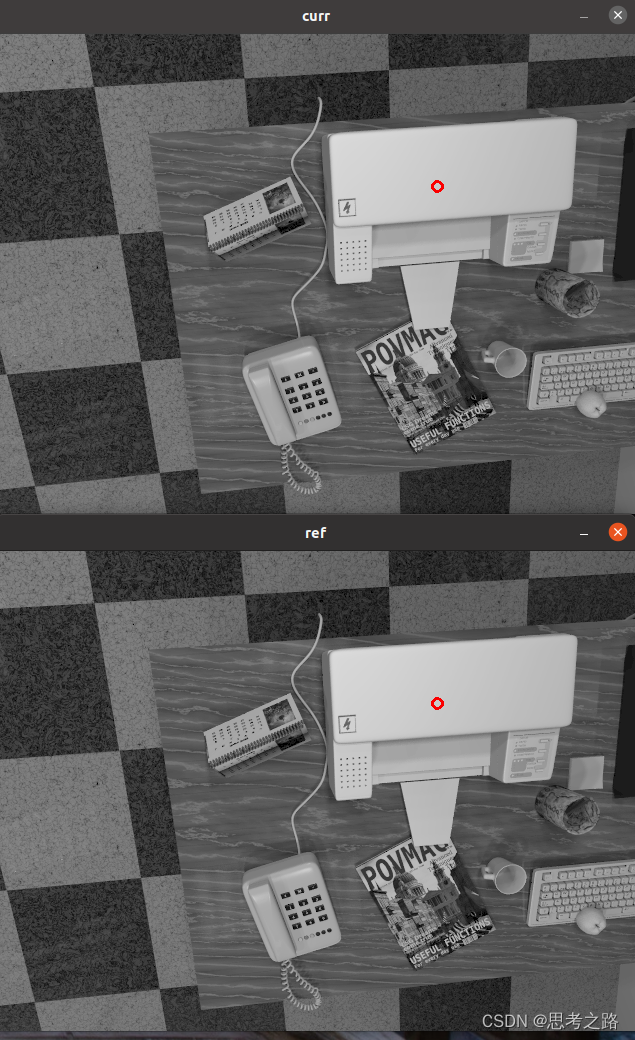
void showEpipolarMatch(const Mat &ref, const Mat &curr, const Vector2d &px_ref, const Vector2d &px_curr) {
    Mat ref_show, curr_show;
    cv::cvtColor(ref, ref_show, CV_GRAY2BGR);
    cv::cvtColor(curr, curr_show, CV_GRAY2BGR);

    cv::circle(ref_show, cv::Point2f(px_ref(0, 0), px_ref(1, 0)), 5, cv::Scalar(0, 0, 250), 2);
    cv::circle(curr_show, cv::Point2f(px_curr(0, 0), px_curr(1, 0)), 5, cv::Scalar(0, 0, 250), 2);

    imshow("ref", ref_show);
    imshow("curr", curr_show);
    waitKey(1);
}

void showEpipolarLine(const Mat &ref, const Mat &curr, const Vector2d &px_ref, const Vector2d &px_min_curr,
                      const Vector2d &px_max_curr) {

    Mat ref_show, curr_show;
    cv::cvtColor(ref, ref_show, CV_GRAY2BGR);
    cv::cvtColor(curr, curr_show, CV_GRAY2BGR);

    cv::circle(ref_show, cv::Point2f(px_ref(0, 0), px_ref(1, 0)), 5, cv::Scalar(0, 255, 0), 2);
    cv::circle(curr_show, cv::Point2f(px_min_curr(0, 0), px_min_curr(1, 0)), 5, cv::Scalar(0, 255, 0), 2);
    cv::circle(curr_show, cv::Point2f(px_max_curr(0, 0), px_max_curr(1, 0)), 5, cv::Scalar(0, 255, 0), 2);
    cv::line(curr_show, Point2f(px_min_curr(0, 0), px_min_curr(1, 0)), Point2f(px_max_curr(0, 0), px_max_curr(1, 0)),
             Scalar(0, 255, 0), 1);

    imshow("ref", ref_show);
    imshow("curr", curr_show);
    waitKey(1);
}

运行结果：由于运行时间比较久，耐心等待。 高博代码中的错误之处：导致无限段错误，原因：
行和列写反了，修改后的结果如下：

Mat depth(width, height, CV_64F, init_depth);             // 深度图
Mat depth_cov2(width, height, CV_64F, init_cov2);         // 深度图方差

整体分析：从数据集中读取了图像，然后交给update函数，对深度进行更新。在update中，我们遍历了参考帧的每个像素，先在当前帧中寻找极线匹配，若匹配上，则利用极线匹配的结果更新深度图的估计。在极线搜索中假设深度服从高斯分布，所以我们以均值为中心，左右各取正负3$\sigma$为半径，在当前帧中寻找极线的投影。然后，遍历此极线上的像素(步长为二分之根号二近似0.7，寻找NCC最高的点作为匹配点，如果最高的NCC也低于阈值0.85，则认为匹配失败。NCC的计算采用了去均值化后的做法，最后进行三角化，不确定性的计算(高斯融合).

1.2 对上述实验的分析和讨论
上述实验演示了移动单目相机的稠密建图，估计了参考帧的每个像素深度。代码相对直接，但并不是最有效的。所以我们可以改进，接下来我们从计算机视觉和滤波器两个角度分析演示实验的结果。
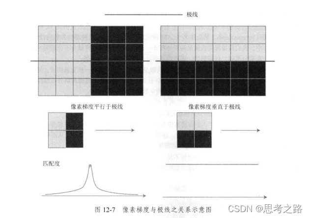
1） 像素梯度的问题
对深度图进行观察中发现，块匹配的正确性与是否依赖于图像块是否就有区分度.所以进行块匹配的时候，必须假设小块不变，然后将该小块与其他小块进行对比。这时有明显梯度的小块具有良好的区分度，不易引起五匹配.对与梯度不明显的像素，由于在块匹配时没有区分性，将难以有效的估计深度。也就是说立体视觉对物体纹理的依赖性强。进一步讨论像素梯度问题，还会发现像素梯度和极线的关系:当像素梯度平行于极线方向，我们能够精确的确定匹配度最高点出现在何处，当像素梯度垂直于极线方向，即使小块有明显的梯度，当我们沿着极线做匹配时，会发现匹配程度都是一样的，得不到有效的匹配。而实际上，梯度与极线的情况有可能介于二者之间：即不完全平行又不完全垂直。也就是说 当像素梯度与极线夹角较大时，极线匹配的不确定性大；当夹角较小时，匹配的不确定性小。

2) 逆深度
逆深度也是一种广泛使用的参数化技巧，在演示程序中，我们假设深度值满足高斯分布d~$N(\mu ,{\sigma }^2)|$,但是真的满足吗，其时不然，最近的点不会小与相机的焦距（或认为深度不小于0),这个分布并不像高斯分布， 形成一个对称的形状。它的尾部可能稍微长，负数区域则为0；而且在一些室外场景，可能存在无穷远的点，初始化中难以涵盖这些点，并且高斯分布描述他们会有一些数值上的困难，于时采用逆深度，深度的倒数，为高斯分布比较有效，也具有更好的数值稳定性,从而成为一种通用的技巧。
3）图像间的变换
在块匹配之前，做一次图像到图像的变换是一种常见的预处理方式。这是因为：我们假设在相机运动时图像小块保持不变，而这个假设在相机平移时能够保持成立，但相机发生旋转后就很难保持成立了。 为了防止这种现象，我们通常在块匹配前，把参考帧和当前帧的运动都参考近来。
参考帧上的一个像素$P_R$与真实三维空间点世界坐标系$P_w$关系：$d_R{P}_R=K(R_{RW}{P}_W+t_{RW})$，类似的当前$P_C$: $d_c{P}_C=K(R_{CW}{P}_W+t_{CW})$, 待入消去$P_W$,即两幅图像间的像素关系为：

当知道$d_R,P_R$时，可以计算出$P_C$的投影位置。此时，再给$P_R$两个分量各一个增量$d_u,d_v$,可以求得$P_C$的增量，算出局部范围内参考帧和当前帧图像坐标变换的一个线性关系构成的仿射变换：

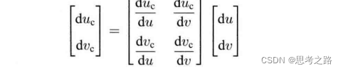根据仿设变换，可以将当前帧的图像进行变换，再进行匹配，以获得对旋转更好的效果。
4）并行化：效率问题
稠密深度图的估计是估计的点从原来数百个特征点变成了图像中所有的像素点，程序的二重循环中遍历了所有的像素，并逐个对他们进行极线搜索，是串行进行的，但是其是每个像素之间是独立的，所以可以并形，利用GPU的稠密深度估计进行可能的加速。
5) 其他改进
各像素是独立的，可能存在某个像素深度很小，边上一个很大的情况。我们可以假设深度图中相邻深度变化不大，从而给深度估计加上了空间正则项。这种做法会使得深度图更加平滑。
我们没有显示的处理外点，由于运动模糊，光照，遮挡等因素的影响，不可能对每个像素都保持成功的匹配。程序中的做法是，只要NCC大于一定的值，就认为匹配成功，没有考虑误匹配的情况。
均匀-高斯分布下的深度滤波器，显式将内点与外点进行区别并进行建模，能够较好的处理外点数据。
使用双目和移动单目相机能够建立稠密的地图，但是过于依赖环境纹理和光照，不可靠。

2 RGB-D稠密建图

在适用的范围内，RGB-D相机是一种更好的选择，可以完全通过传感器中硬件的测量得到深度值，而且深度相机的结构光或飞时原理，保证了深度数据对纹理的无关性。即使是纯色物体，只要能过反射光，就能测到它的深度。
根据地图形式的不同，也存在多种不同的主流建图方式。最直观的就是根据估算的相机位姿，将RGB-D数据转为点云，然后拼接，最后得到一个由离散的点组成的点云地图。如果我们还要对外观有要求，希望估计物体的表面，则使用三角网格，面片进行建图。如果希望知道地图的障碍物信息并在地图上导航，可以使用体素建立占据网格地图。
实战：点云地图
点云地图中的每个点包含x,y,z,r,g, b信息。RGB-D提供了彩色图和深度图，因此很容易用相机内参计算RGB-D点云。通过某种手段得到相机的位姿，那么只要直接把点云进行加权，就可以获得全局的点云。而在实际的建图中，我们还会对点云加一些滤波处理，以获得更好的视觉效果。主要使用的两种滤波器：外点去除滤波器，体素网格的降采样滤波器。
程序代码：

#include <iostream>
#include <fstream>

using namespace std;

#include <opencv2/core/core.hpp>
#include <opencv2/highgui/highgui.hpp>
#include <Eigen/Geometry>
#include <boost/format.hpp>  // for formating strings
#include <pcl/point_types.h>
#include <pcl/io/pcd_io.h>
#include <pcl/filters/voxel_grid.h>
#include <pcl/visualization/pcl_visualizer.h>
#include <pcl/filters/statistical_outlier_removal.h>

int main(int argc, char **argv) {
    vector<cv::Mat> colorImgs, depthImgs;    // 彩色图和深度图
    vector<Eigen::Isometry3d> poses;         // 相机位姿

    ifstream fin("./data/pose.txt");
    if (!fin) {
        cerr << "cannot find pose file" << endl;
        return 1;
    }

    for (int i = 0; i < 5; i++) {
        boost::format fmt("./data/%s/%d.%s"); //图像文件格式
        colorImgs.push_back(cv::imread((fmt % "color" % (i + 1) % "png").str()));
        depthImgs.push_back(cv::imread((fmt % "depth" % (i + 1) % "png").str(), -1)); // 使用-1读取原始图像

        double data[7] = {0};
        for (int i = 0; i < 7; i++) {
            fin >> data[i];
        }
        Eigen::Quaterniond q(data[6], data[3], data[4], data[5]);
        Eigen::Isometry3d T(q);
        T.pretranslate(Eigen::Vector3d(data[0], data[1], data[2]));
        poses.push_back(T);
    }

    // 计算点云并拼接
    // 相机内参 
    double cx = 319.5;
    double cy = 239.5;
    double fx = 481.2;
    double fy = -480.0;
    double depthScale = 5000.0;

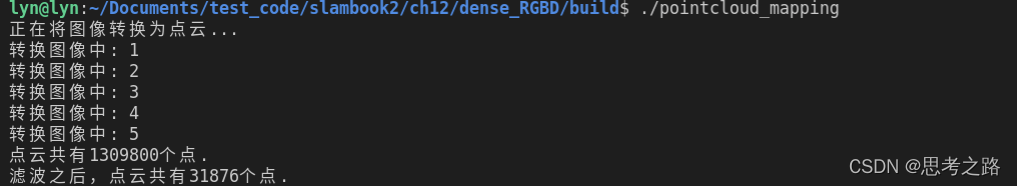
    cout << "正在将图像转换为点云..." << endl;

    // 定义点云使用的格式：这里用的是XYZRGB
    typedef pcl::PointXYZRGB PointT;
    typedef pcl::PointCloud<PointT> PointCloud;

    // 新建一个点云
    PointCloud::Ptr pointCloud(new PointCloud);
    for (int i = 0; i < 5; i++) {
        PointCloud::Ptr current(new PointCloud);
        cout << "转换图像中: " << i + 1 << endl;
        cv::Mat color = colorImgs[i];
        cv::Mat depth = depthImgs[i];
        Eigen::Isometry3d T = poses[i];
        for (int v = 0; v < color.rows; v++)
            for (int u = 0; u < color.cols; u++) {
                unsigned int d = depth.ptr<unsigned short>(v)[u]; // 深度值
                if (d == 0) continue; // 为0表示没有测量到
                Eigen::Vector3d point;
                point[2] = double(d) / depthScale;
                point[0] = (u - cx) * point[2] / fx;
                point[1] = (v - cy) * point[2] / fy;
                Eigen::Vector3d pointWorld = T * point;

                PointT p;
                p.x = pointWorld[0];
                p.y = pointWorld[1];
                p.z = pointWorld[2];
                p.b = color.data[v * color.step + u * color.channels()];
                p.g = color.data[v * color.step + u * color.channels() + 1];
                p.r = color.data[v * color.step + u * color.channels() + 2];
                current->points.push_back(p);
            }
        // depth filter and statistical removal 
        PointCloud::Ptr tmp(new PointCloud);
        pcl::StatisticalOutlierRemoval<PointT> statistical_filter;//去掉深度值无效的点
        statistical_filter.setMeanK(50); //过滤掉孤立的点
        statistical_filter.setStddevMulThresh(1.0); 
        statistical_filter.setInputCloud(current);
        statistical_filter.filter(*tmp);
        (*pointCloud) += *tmp;
    }

    pointCloud->is_dense = false;
    cout << "点云共有" << pointCloud->size() << "个点." << endl;

    // voxel filter 体素网格滤波器
    pcl::VoxelGrid<PointT> voxel_filter;
    double resolution = 0.03;  //体素网格滤波器的分辨率0.003 x 0.003 x 0.003
    voxel_filter.setLeafSize(resolution, resolution, resolution);       // resolution
    PointCloud::Ptr tmp(new PointCloud);
    voxel_filter.setInputCloud(pointCloud);
    voxel_filter.filter(*tmp);
    tmp->swap(*pointCloud);

    cout << "滤波之后，点云共有" << pointCloud->size() << "个点." << endl;

    pcl::io::savePCDFileBinary("map.pcd", *pointCloud);
    return 0;
}

本实验的数据集使用ICL-NUIM数据集。
需要使用pcl工具：sudo apt-get install libpcl-dev plc-tools进行点云库的安装。
代码使用滤波器的地方讲解：
1）在生成每帧点云时，去掉深度值无效的点。这主要是考虑Kinect的有效量程，超过有效量程后的深度会有较大的误差或返回一个零。
2）利用嗯统计滤波器方法去除孤立点。该滤波器统计每个点与它最近的N个点的距离值的分布，去除距离均值过大的点。去除了孤立噪声点。
3）利用体素网格滤波器进行降采样。由于多个视角存在视野重叠，在重叠区域会存在大量的位置十分相近的点。会占据内存空间。体素滤波器保证了在某个一定大小的立方体(体素)内仅有一个点，相当于对三维空间进行了降采样，从而节省了存储空间。
在体素滤波器中，我们把分辨率设成0.03，表示每个0.03x0.03x0.03的立方体中只有一个点，这个分辨率较高，所以实际中感觉不到地图的差异，单程序输出中点数明显减少。
CMakeLists.txt:

cmake_minimum_required(VERSION 3.4)

set(CMAKE_BUILD_TYPE Release)
set(CMAKE_CXX_FLAGS "-std=c++14 -O2")

# opencv 
find_package(OpenCV 3.4 REQUIRED)
include_directories(${OpenCV_INCLUDE_DIRS})

# eigen 
include_directories("/usr/include/eigen3/")

# pcl 
find_package(PCL REQUIRED)
include_directories(${PCL_INCLUDE_DIRS})
add_definitions(${PCL_DEFINITIONS})

add_executable(pointcloud_mapping pointcloud_mapping.cpp)
target_link_libraries(pointcloud_mapping ${OpenCV_LIBS} ${PCL_LIBRARIES})

运行结果：


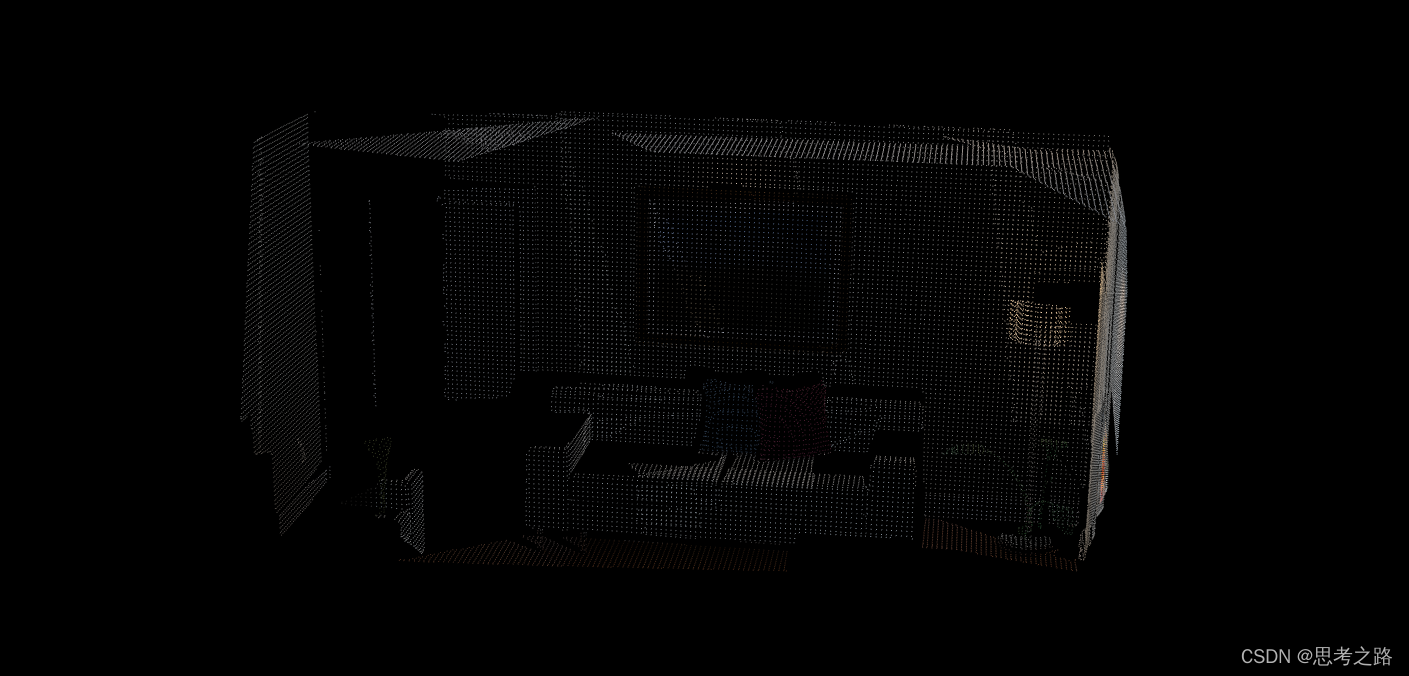
点云地图可直接由RGB-D图像高效生成，无需格外处理，不过，点云表达的地图是十分初级的，而我们希望的地图往往是能满足以下要求的：
1）定位：取决与前端视觉里程计的处理方式。如果是基于特征点的视觉里程计，由于点云中没有存储特征点的信息，则无法用于基于特征点的定位方式。如果前端是点云的ICP，那么可以将局部点云对全局点云进行ICP以估计位姿。
2）导航与避障:点云无法直接用于避障，纯粹的点云无法表示“是否有障碍物",不过，可以在点云的基础上加工，得到更适合导航避障的地图形式。
3）可视化和交互:点云只有离散的点，没有物体表面的信息，所以不符合可视化要求。
点云是基础的，初级的，接近传感器读取的原始数据，更高级的功能，如导航避障，可以从点云出发，构建占据网格地图,以供导航算法查询某点是否能通过。SfM中常使用的柏松重建，就能通过基本的点云重建物体网格地图，得到物体的表面信息。还有Surfel也是一种表达物体表面的方式，以面元作为地图的基本单位，能建立可视化地图。
大部分由点云转换得到的地图形式都在PCL库中提供。

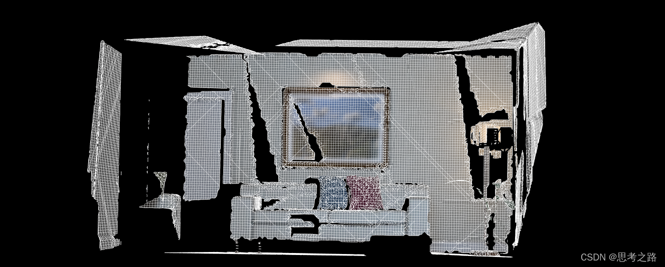
实战：从点云重建网格
思路：先计算点云的法线，在从法线计算网格。
class pcl: : MovingLeastSquares< PointlnT, PointOutT>
类 MovingLeastSquares 实现了基于移动最小二乘算法的点云平滑处理、数据重采样，并且可以计算优化的估计法线，其输入是点云数据，输出为经过用户设定参数对应的处理之后得到的平滑重采样点云
实现代码：

//
// Created by gaoxiang on 19-4-25.
//

#include <pcl/point_cloud.h>
#include <pcl/point_types.h>  //PCL对各种格式的点的支持头文件
#include <pcl/io/pcd_io.h>  //PCL的PCD格式文件输入输出头文件
#include <pcl/visualization/pcl_visualizer.h>
#include <pcl/kdtree/kdtree_flann.h>
#include <pcl/surface/surfel_smoothing.h>
#include <pcl/surface/mls.h>
#include <pcl/surface/gp3.h>
#include <pcl/surface/impl/mls.hpp>

// typedefs
typedef pcl::PointXYZRGB PointT;
typedef pcl::PointCloud<PointT> PointCloud;
typedef pcl::PointCloud<PointT>::Ptr PointCloudPtr;
typedef pcl::PointXYZRGBNormal SurfelT;
typedef pcl::PointCloud<SurfelT> SurfelCloud;
typedef pcl::PointCloud<SurfelT>::Ptr SurfelCloudPtr;

SurfelCloudPtr reconstructSurface(
        const PointCloudPtr &input, float radius, int polynomial_order) {
    pcl::MovingLeastSquares<PointT, SurfelT> mls; //PointT决定了输入点云类型，SurfelT决定了输出点云类型(当法线标志位设置为true时，输出向量必须加上normals)  点云重建算法Moving Least Square
    pcl::search::KdTree<PointT>::Ptr tree(new pcl::search::KdTree<PointT>);
    mls.setSearchMethod(tree); //使用kdTree加速搜索
    mls.setSearchRadius(radius);  //设置搜索半径 radius ，确定多项式拟合时所用的邻域点进行 k 近邻搜索时所用的半径。
    mls.setComputeNormals(true);  //设置是否计算并存储点云对应的法线，参数为 true 则设置为是。
    mls.setSqrGaussParam(radius * radius);//设置近邻高斯权重系数 sqr_ gauss_ param ， 一般设置成搜索半径的平方时效果最好
    mls.setPolynomialFit(polynomial_order > 1);//设置在进行估计法线时是否使用多项式拟合进行逼近，还是仅通过切线估计得到， polynomial_ fit 参数为 true 则设置为是 。
    mls.setPolynomialOrder(polynomial_order);//设置使用多项式拟合进行运算时所用的阶数 order .
    mls.setInputCloud(input);  //输入需要进行平滑滤波处理的点云
    SurfelCloudPtr output(new SurfelCloud);
    mls.process(*output);  //输出处理后的点云
    return (output);
}

pcl::PolygonMeshPtr triangulateMesh(const SurfelCloudPtr &surfels) {
    // Create search tree*
    pcl::search::KdTree<SurfelT>::Ptr tree(new pcl::search::KdTree<SurfelT>);
    tree->setInputCloud(surfels);

    // Initialize objects
    pcl::GreedyProjectionTriangulation<SurfelT> gp3;
    pcl::PolygonMeshPtr triangles(new pcl::PolygonMesh);

    // Set the maximum distance between connected points (maximum edge length)
    gp3.setSearchRadius(0.05);

    // Set typical values for the parameters
    gp3.setMu(2.5);
    gp3.setMaximumNearestNeighbors(100);
    gp3.setMaximumSurfaceAngle(M_PI / 4); // 45 degrees
    gp3.setMinimumAngle(M_PI / 18); // 10 degrees
    gp3.setMaximumAngle(2 * M_PI / 3); // 120 degrees
    gp3.setNormalConsistency(true);

    // Get result
    gp3.setInputCloud(surfels);
    gp3.setSearchMethod(tree);
    gp3.reconstruct(*triangles);

    return triangles;
}

int main(int argc, char **argv) {

    // Load the points
    PointCloudPtr cloud(new PointCloud);  //创建点云指针
    if (argc == 0 || pcl::io::loadPCDFile(argv[1], *cloud)) {  //读入PCD格式的文件
        cout << "failed to load point cloud!";
        return 1;
    }
    cout << "point cloud loaded, points: " << cloud->points.size() << endl;

    // Compute surface elements
    cout << "computing normals ... " << endl;
    double mls_radius = 0.05, polynomial_order = 2;
    auto surfels = reconstructSurface(cloud, mls_radius, polynomial_order);

    // Compute a greedy surface triangulation
    cout << "computing mesh ... " << endl;
    pcl::PolygonMeshPtr mesh = triangulateMesh(surfels); //两个相机位姿和特征点在两个相机坐标系下的坐标，输出三角化后的特征点的3D坐标。

    cout << "display mesh ... " << endl;
    pcl::visualization::PCLVisualizer vis;
    vis.addPolylineFromPolygonMesh(*mesh, "mesh frame");
    vis.addPolygonMesh(*mesh, "mesh");
    vis.resetCamera();
    vis.spin();
}

执行：./sufel_mapping map.pcd
实现效果：

八叉树地图
八叉树地图：是在导航中常用的，本身有较好压缩性能的地图形式。
在点云地图中，我们虽然有了三维结构，也进行了体素滤波器以调整分辨率，但是点云有几个明显的缺点：

• 点云规模大，所以pcd文件也很大，640x480图像上有30万个点空间，需要大量存储空间。进过体素滤波后，还是很大，点云地图提供了一些细节(阴影)等，但是放在有限的空间中浪费，我们只要降低分辨率，才能在有限的空间中存储大规模环境，但是降低分辨率会导致图像质量下降。需要一种对图像进行压缩，可以舍弃重复信息的地图形式

• 点云地图无法处理运动物体。我们只能添加点，而没有“当点消失时把它移除”的做法。在实际的环境中，运动物体的普遍存在，使得点云地图变得不够实用。

  三维空间建模为许多个小方块(体素)是一种常见方法。如果我们把一个小方块的每个面平均切成两片，那末每个小方块就变成同样大小的八个小方块。这个步骤可以不断重复，知道最后的方块大小达到建模的最高精度,。在这个过程中，把一个方块分成8个大小一样的小方块看成“一个节点展开成8个子节点”， 那么整个最大空间细到最小空间的过程，就是一个八叉树。
  如叶子节点立方体大小为1， 10层树，建模体积大约是8的10次方 ——1073
  
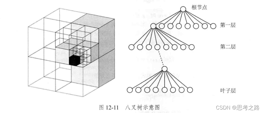
  点云比八叉数占空间：**在八叉数中，在节点中存储它是否被占据的信息。当某个方块的所有子节点都被占据或不被占据时，就没必要展开这个节点。**例如：当地图一开始是空白，只有一个根节点，不需要完成的树，当向地图中添加信息时，由于实际的物体经常连在一起，空白的地方也连在一起，所以八叉树无需展开到叶子节点。
  假设用一个浮点数x [0, 1]来表达，一开始取0.5 , 如果不断的观测到它被占据，就让这个值不断增加，反之，如果不断观测到空白，就让他不断减小。通过这种方式，可以动态的建模地图中的障碍信息。不过，由于x的增加或减少会超出范围（其中0 或1 是占据或不被占据的含义，中间值是由于噪声影响会出现未知的情况)，所以不直接用概率描述节点是否被占据，而用概率对数值来描述。
  y是概率对数值，x是0～1的概率，他们的变换由logit变换来描述：
  
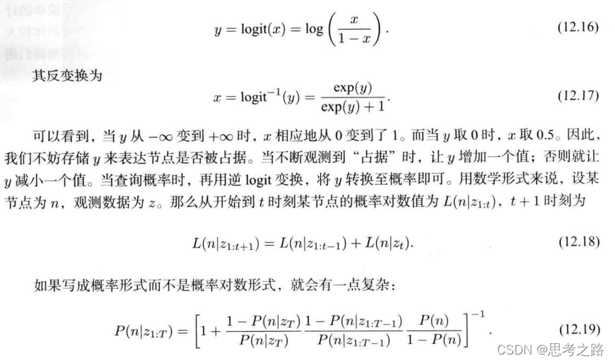
  有了对数概率，就可以根据RGB-D数据更新整个八叉树地图了。假设RGB-D图像中观测到某个像素带有深度d，就说明:在深度值对应的空间点上观察到了一个占据数据，并且，从相机光心出发到这个点的线段上应该是没有物体的(否则被遮挡)。利用这个信息，可以对八叉树进行更新，并且能处理运动的结构。
  实例：八叉树地图
  安装octmap库，八叉树地图和对应的可视化工具octovis在该库中：sudo apt-get install liboctomap-dev octovis
  实现代码：

#include <iostream>
#include <fstream>

using namespace std;

#include <opencv2/core/core.hpp>
#include <opencv2/highgui/highgui.hpp>

#include <octomap/octomap.h>    // for octomap 

#include <Eigen/Geometry>
#include <boost/format.hpp>  // for formating strings

int main(int argc, char **argv) {
    vector<cv::Mat> colorImgs, depthImgs;    // 彩色图和深度图
    vector<Eigen::Isometry3d> poses;         // 相机位姿

    ifstream fin("../data/pose.txt");
    if (!fin) {
        cerr << "cannot find pose file" << endl;
        return 1;
    }

    for (int i = 0; i < 5; i++) {
        boost::format fmt("../data/%s/%d.%s"); //图像文件格式
        colorImgs.push_back(cv::imread((fmt % "color" % (i + 1) % "png").str()));
        depthImgs.push_back(cv::imread((fmt % "depth" % (i + 1) % "png").str(), -1)); // 使用-1读取原始图像

        double data[7] = {0};
        for (int i = 0; i < 7; i++) {
            fin >> data[i];
        }
        Eigen::Quaterniond q(data[6], data[3], data[4], data[5]);
        Eigen::Isometry3d T(q);
        T.pretranslate(Eigen::Vector3d(data[0], data[1], data[2]));
        poses.push_back(T);
    }

    // 计算点云并拼接
    // 相机内参 
    double cx = 319.5;
    double cy = 239.5;
    double fx = 481.2;
    double fy = -480.0;
    double depthScale = 5000.0;

    cout << "正在将图像转换为 Octomap ..." << endl;

    // octomap tree 
    octomap::OcTree tree(0.01); // 参数为分辨率

    for (int i = 0; i < 5; i++) {
        cout << "转换图像中: " << i + 1 << endl;
        cv::Mat color = colorImgs[i];
        cv::Mat depth = depthImgs[i];
        Eigen::Isometry3d T = poses[i];

        octomap::Pointcloud cloud;  // the point cloud in octomap 

        for (int v = 0; v < color.rows; v++)
            for (int u = 0; u < color.cols; u++) {
                unsigned int d = depth.ptr<unsigned short>(v)[u]; // 深度值
                if (d == 0) continue; // 为0表示没有测量到
                Eigen::Vector3d point;
                point[2] = double(d) / depthScale;
                point[0] = (u - cx) * point[2] / fx;
                point[1] = (v - cy) * point[2] / fy;
                Eigen::Vector3d pointWorld = T * point;
                // 将世界坐标系的点放入点云
                cloud.push_back(pointWorld[0], pointWorld[1], pointWorld[2]);
            }

        // 将点云存入八叉树地图，给定原点，这样可以计算投射线
        tree.insertPointCloud(cloud, octomap::point3d(T(0, 3), T(1, 3), T(2, 3)));
    }

    // 更新中间节点的占据信息并写入磁盘
    tree.updateInnerOccupancy();
    cout << "saving octomap ... " << endl;
    tree.writeBinary("octomap.bt");
    return 0;
}

运行结果：

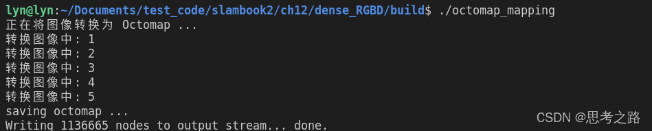
octovis octomap.bt命令进行 可视化查看：按“1”键可以根据高度信息进行染色。

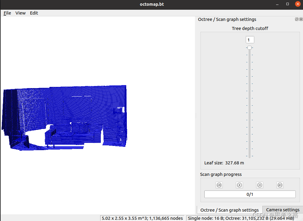
使用octomap::OcTree构建整张地图。内部提供了一个点云结构，但比PCL的点云简单，只携带点的空间位置信息。我们根据RGB-D图像和相机位姿信息，先将点点坐标转到世界坐标，然后放入八叉树地图的点云，最后交给八叉树地图。我们把生成的地图存成octmap.bt文件。