2025年美赛C题：奥运奖牌榜模型27种模型Python代码2000行+的全网最详细代码

本文链接：https://blog.csdn.net/weixin_43935696/article/details/145347636

题目和背景

见另一篇博客

2025年美赛C题：奥运奖牌榜模型解析及Python代码实现

完整代码获取见Github：https://github.com/cityu-lm/2025_MCM_Problem_C

1. 引言

根据记录了120年奥运会数据的公共数据集，并将其转换为包含以下特征的数据集：国家、年份、运动、赛事、人口、GDP、年龄、BMI、身高、体重、性别和季节。目标变量是获得的奖牌类型，包括无奖牌、铜牌、银牌或金牌，使用监督分类机器学习模型来预测哪些运动员将获得哪些奖牌。此外，使用Label Encoding和One Hot Encoding对分类数据进行了转换，并使用对数转换、最小最大标量和标准标量对数据进行了缩放。为了平衡的目标变量，使用随机重采样和SMOTE进行重采样。然后，使用k近邻、朴素贝叶斯和决策树分类器对的测试数据进行特征选择和超参数调优。的结果显示了一个成功的模型使用SMOTE采样，没有特征选择和超参数调优的kNN。

通过以下分析，将能够了解这种差异是否显著，或者其他因素，如运动员的身高和体重，是否对他们的表现更有影响。从某种意义上说，希望的分析可以为各国如何挑选运动员提供见解，理想情况下，可以找出历史上在奥运会上表现最差的国家，以及为什么会这样。

2. 方法

数据集是关于120年来奥运会运动员和他们在各种项目中的表现。删除带有NaN值的行后，的数据集包含206,165行。这样做是为了得到只包含完整数据的样本。从该数据集中获得的特征包括性别、年龄、身高、体重、年份、国家、季节、运动、赛事和奖牌。删除了一些认为不会影响模型或冗余的功能，如团队（以国家名称表示）、游戏（以年份和赛季表示）以及不会影响运动员表现的名称。还添加了BMI特征，它是根据的身高和体重值计算出来的，以便将来研究它与其他特征的相关性。此外，为了确定运动员所在国家的GDP是否会影响他们的表现，将每个国家的GDP和人口（来自GeoPandas模块）添加到的数据集中。的目标变量是在比赛中获得的奖牌（金、银、铜或无）。

数据集在目标变量方面并不平衡，因为正如预期的那样，在目标变量中标记为“无”（意味着他们没有赢得奖牌）的样本明显多于标记为“铜”，“银”和“金”的样本。85.4%的样本被归为无奖牌（175,984个样本），4.8%的样本被归为金牌（10,167个样本），4.9%的样本被归为银牌（9,866个样本），4.9%的样本被归为铜牌（10,148个样本）。比较了两种不同的重新抽样方法的结果：抽样并因此将所有目标计数更改为9,800，并使用SMOTE对的少数类别（青铜，白银和黄金）进行抽样，将所有目标计数更改为175,739，或原始计数为None。

2.1.1 数据导入

请添加图片描述

在本节中，首先从csv文件导入数据。然后，通过删除空值、删除不打算使用的列（即国家代码、运动员id）以及重命名一些列来清理数据（将原始的“Medal”列设置为目标列）。

import pandas as pd
import numpy as np
import matplotlib.pyplot as plt
import seaborn as sns
import geopandas as gpd
# pip install geopandas
%matplotlib inline

# Import olympic athletes dataset
athletes_url = "data/athlete_events.csv"

df_athletes = pd.read_csv(athletes_url)
df_athletes

	ID	Name	Sex	Age	Height	Weight	Team	NOC	Games	Year	Season	City	Sport	Event	Medal
0	1	A Dijiang	M	24.0	180.0	80.0	China	CHN	1992 Summer	1992	Summer	Barcelona	Basketball	Basketball Men's Basketball	NaN
1	2	A Lamusi	M	23.0	170.0	60.0	China	CHN	2012 Summer	2012	Summer	London	Judo	Judo Men's Extra-Lightweight	NaN
2	3	Gunnar Nielsen Aaby	M	24.0	NaN	NaN	Denmark	DEN	1920 Summer	1920	Summer	Antwerpen	Football	Football Men's Football	NaN
3	4	Edgar Lindenau Aabye	M	34.0	NaN	NaN	Denmark/Sweden	DEN	1900 Summer	1900	Summer	Paris	Tug-Of-War	Tug-Of-War Men's Tug-Of-War	Gold
4	5	Christine Jacoba Aaftink	F	21.0	185.0	82.0	Netherlands	NED	1988 Winter	1988	Winter	Calgary	Speed Skating	Speed Skating Women's 500 metres	NaN
...	...	...	...	...	...	...	...	...	...	...	...	...	...	...	...
271111	135569	Andrzej ya	M	29.0	179.0	89.0	Poland-1	POL	1976 Winter	1976	Winter	Innsbruck	Luge	Luge Mixed (Men)'s Doubles	NaN
271112	135570	Piotr ya	M	27.0	176.0	59.0	Poland	POL	2014 Winter	2014	Winter	Sochi	Ski Jumping	Ski Jumping Men's Large Hill, Individual	NaN
271113	135570	Piotr ya	M	27.0	176.0	59.0	Poland	POL	2014 Winter	2014	Winter	Sochi	Ski Jumping	Ski Jumping Men's Large Hill, Team	NaN
271114	135571	Tomasz Ireneusz ya	M	30.0	185.0	96.0	Poland	POL	1998 Winter	1998	Winter	Nagano	Bobsleigh	Bobsleigh Men's Four	NaN
271115	135571	Tomasz Ireneusz ya	M	34.0	185.0	96.0	Poland	POL	2002 Winter	2002	Winter	Salt Lake City	Bobsleigh	Bobsleigh Men's Four	NaN

271116 rows × 15 columns

# Read country codes data file
noc_url = "data/noc_regions.csv"
noc = pd.read_csv(noc_url)
noc

	NOC	region	notes
0	AFG	Afghanistan	NaN
1	AHO	Curacao	Netherlands Antilles
2	ALB	Albania	NaN
3	ALG	Algeria	NaN
4	AND	Andorra	NaN
...	...	...	...
225	YEM	Yemen	NaN
226	YMD	Yemen	South Yemen
227	YUG	Serbia	Yugoslavia
228	ZAM	Zambia	NaN
229	ZIM	Zimbabwe	NaN

230 rows × 3 columns

# Read world shape file from github link for gdp and population features
world_url = "https://github.com/emily-ywang/Olympics-ML-Project/blob/master/world.csv?raw=true"
world = pd.read_csv(world_url)

world

	Unnamed: 0	OBJECTID	featurecla	LEVEL	TYPE	FORMAL_EN	FORMAL_FR	POP_EST	POP_RANK	GDP_MD_EST	...	NAME_SV	NAME_TR	NAME_VI	NAME_ZH	WB_NAME	WB_RULES	WB_REGION	Shape_Leng	Shape_Area	geometry
0	0	1	Admin-0 country	2	Sovereign country	Republic of Indonesia	NaN	260580739	17	3028000.0	...	Indonesien	Endonezya	Indonesia	印度尼西亚	Indonesia	None	EAP	495.029918	153.078608	MULTIPOLYGON (((117.7036079042814 4.1634145420...
1	1	2	Admin-0 country	2	Sovereign country	Malaysia	NaN	31381992	15	863000.0	...	Malaysia	Malezya	Malaysia	马来西亚	Malaysia	None	EAP	68.456913	26.703172	MULTIPOLYGON (((117.7036079042814 4.1634145420...
2	2	3	Admin-0 country	2	Sovereign country	Republic of Chile	NaN	17789267	14	436100.0	...	Chile	Şili	Chile	智利	Chile	None	LCR	416.997272	76.761813	MULTIPOLYGON (((-69.51008875159459 -17.5065881...
3	3	4	Admin-0 country	2	Sovereign country	Plurinational State of Bolivia	NaN	11138234	14	78350.0	...	Bolivia	Bolivya	Bolivia	玻利維亞	Bolivia	None	LCR	54.345991	92.203587	POLYGON ((-69.51008875159459 -17.5065881976871...
4	4	5	Admin-0 country	2	Sovereign country	Republic of Peru	NaN	31036656	15	410400.0	...	Peru	Peru	Peru	秘鲁	Peru	None	LCR	73.262192	106.417089	MULTIPOLYGON (((-69.51008875159459 -17.5065881...
...	...	...	...	...	...	...	...	...	...	...	...	...	...	...	...	...	...	...	...	...	...
246	246	247	Admin-0 country	2	Dependency	NaN	NaN	300	2	0.0	...	Förenta staternas mindre öar i Oceanien och Vä...	United States Minor Outlying Islands	Các tiểu đảo xa của Hoa Kỳ	美国本土外小岛屿	Navassa Island (US)	Name in italic	Other	0.085608	0.000413	POLYGON ((-75.02432206870844 18.41726308762145...
247	247	248	Admin-0 country	2	Dependency	NaN	NaN	300	2	0.0	...	Förenta staternas mindre öar i Oceanien och Vä...	United States Minor Outlying Islands	Các tiểu đảo xa của Hoa Kỳ	美国本土外小岛屿	Palmyra Atoll (US)	Name in italic	Other	0.147363	0.000576	POLYGON ((-162.0608617830448 5.88719310098088,...
248	248	249	Admin-0 country	2	Dependency	NaN	NaN	300	2	0.0	...	Förenta staternas mindre öar i Oceanien och Vä...	United States Minor Outlying Islands	Các tiểu đảo xa của Hoa Kỳ	美国本土外小岛屿	Kingman Reef (US)	Name in italic	Other	0.059570	0.000222	POLYGON ((-162.4001765620986 6.445135808770601...
249	249	250	Admin-0 country	2	Country	New Zealand	NaN	4510327	12	174800.0	...	Nya Zeeland	Yeni Zelanda	New Zealand	新西兰	Tokelau (NZ)	Name in italic	Other	0.178453	0.000348	MULTIPOLYGON (((-171.1856583318665 -9.36126067...
250	250	251	Admin-0 country	2	Country	New Zealand	NaN	4510327	12	174800.0	...	Nya Zeeland	Yeni Zelanda	New Zealand	新西兰	New Zealand	None	Other	104.828986	29.143542	MULTIPOLYGON (((169.2127597908318 -52.47456229...

251 rows × 54 columns

world.to_csv('data/world.csv',index=False)

2.2. 数据分析

根据国家、年份、运动项目、赛事、人口、GDP、年龄、BMI、身高、体重、性别和季节等特征来预测奥运会运动员获得的奖牌（无、铜、银或金）。县，GDP和人口是重要的特征，因为许多国家比其他国家在奥运会上表现得更好，因为他们的规模，因为较高的人口通常有更多的机会培养优秀的运动员，而GDP影响了获得体育资金和资源的机会。所有这三个因素都表明，某些国家，主要是第一世界国家，在奥运会上的表现要好于资源较少的国家。此外，某些国家在某些项目上比其他国家更擅长，例如，非洲的一个国家可能不擅长滑雪，但赤道以上的一个国家在冬天经常下雪，可能更擅长滑雪。因此，体育和项目是重要的特征，因为某些国家在某些项目上表现更好，某些人根据他们的身高、体重、年龄、性别和BMI可能在这些项目或运动中表现更好。BMI、身高、体重、性别和年龄告诉运动员的个人特征；它们很重要，因为这些差异在决定运动员能否获得奖牌方面起着重要作用。年份是一个重要的特征，因为总的来说，奥运会和田径运动发生了很多变化，的数据集可以追溯到很久以前。有些项目已经不存在了，有些项目是多年来增加的。最后，季节是一个重要的特征，因为在夏季奥运会上获得奖牌的机会比冬季奥运会要多，所以的模型在预测运动员获得奖牌时需要考虑到这一点。

这是一个有监督的机器学习问题，因为的数据集是有标签的，从这些标签中，的模型预测运动员获得了什么奖牌（无，铜牌，银牌或金牌）。的标签包含有关运动员的信息，包括他们的身体信息，他们的国家，他们参加的比赛。利用这些信息和已知的目标变量结果，的模型可以预测目标变量。的项目处理一个分类问题，因为使用年龄、身高、体重和项目等特征来训练的模型，并给出一组相应的特征，对运动员最有可能赢得的奖牌类型（铜牌、银牌、金牌或没有奖牌）进行分类。

在数据上使用了k近邻、朴素贝叶斯和决策树。选择这些是因为它们处理监督分类机器学习问题。具体来说，选择k-Nearest Neighbors是因为对于分类问题，它的性能很好，需要做的调整很少，而且由于没有太多的特征，所以效果很好。选择朴素贝叶斯是因为它是一种具有有效参数估计的概率分类算法，然而，预计其他算法可能会更好地泛化。最后，选择决策树，因为的数据集包含不同的特征类型，而决策树特别擅长对不同的数据类型进行分类，并且决策树易于理解。

3. 实验结果

3.1. 数据分析

3.1.1 数据清洗：运动员数据集

在下面的单元格中，在除“Medal”之外的任何列中删除了具有Na值的样本，因为这些缺失的值可能会在处理和操作数据集时导致复杂性。在的目标变量“奖牌”一栏中，NA值代表没有奖牌，而不是一个缺失值；因此，将“Medal”中的所有NA值替换为字符串none，表示该运动员没有获得奖牌。

# Drop null values (except for Medal) and sort by year
df_athletes.dropna(subset=['ID', 'Name', 'Sex', 'Age', 'Height', 'Weight', 'Team', 'NOC', 
                         'Games', 'Year', 'Season', 'City', 'Sport', 'Event'], inplace=True)
df_athletes.sort_values('Year', inplace=True)

# Change remaining Nan values in medal column to be 'None'
df_athletes.replace(np.nan, 'None', regex=True, inplace=True)

# Rename "Medal" column as target
df_athletes.rename(columns={"Medal":"target"}, inplace=True)

3.1.2 数据清理和合并数据框架：NOC数据集

在下面的单元格中，将初始数据框（包含名称、NOC（国家代码名称）、年龄、身高、体重等）与包含国家名称（NOC）代码以及每个国家的全名的数据框合并，以便的最终数据框包含每个国家的全名而不是国家代码。然后，删除了不会影响运动员成绩的列，如Name、City、ID，以及冗余的列，如NOC、Teams和Games。

# Combine NOC region names with NOC codes in dataset
merged = pd.merge(df_athletes, noc, how='inner')
df_data = merged.rename(columns={'region': 'Country'})

# Drop redundant columns (Name, ID, NOC, Games, Sport, notes, City)
df_data.drop(['Name', 'ID', 'NOC', 'Team', 'Games', 'notes', 'City'], axis=1, inplace=True)

3.1.3 数据清理和合并数据框架：世界数据集

import warnings
warnings.filterwarnings('ignore')
# Limit world dataset to three columns: country name, population, and GDP
df_world = world[['NAME_EN', 'POP_EST', 'GDP_MD_EST']]
df_world.rename(columns={'NAME_EN':'Country', 'POP_EST':'Population', 'GDP_MD_EST':'GDP'}, inplace=True)

# Replace country names that don't match with noc names
df_world.replace({'Country':{"People's Republic of China":"China", "United Kingdom":"UK", 
                          "United States of America":"USA", "The Bahamas":"Bahamas",
                         "Trinidad and Tobago":"Trinidad"}}, inplace=True)

在下面的单元格中，将数据集与包含每个国家的GDP和人口数据的数据集合并。

# Rename "Taiwan" country rows as "China" (world dataset only has China, not Taiwan)
df_data.replace({"Country":"Taiwan"}, "China", inplace=True)

# Reorder columns
df_data = df_data[['Sex', 'Age', 'Height', 'Weight', 'Year', 'Country', 'Season', 'Sport', 'Event', 'target']]

# Reset index
df_data.reset_index(drop=True, inplace=True)

# Merge world dataset with athletes dataset
df_data = df_world.merge(df_data)

3.1.4 清理和合并数据集

df_data

	Country	Population	GDP	Sex	Age	Height	Weight	Year	Season	Sport	Event	target
0	Indonesia	260580739	3028000.0	M	20.0	162.0	57.0	1956	Summer	Athletics	Athletics Men's 100 metres	None
1	Indonesia	260580739	3028000.0	M	22.0	160.0	56.0	1960	Summer	Weightlifting	Weightlifting Men's Bantamweight	None
2	Indonesia	260580739	3028000.0	M	37.0	172.0	70.0	1960	Summer	Sailing	Sailing Mixed Three Person Keelboat	None
3	Indonesia	260580739	3028000.0	M	18.0	172.0	66.0	1960	Summer	Cycling	Cycling Men's 100 kilometres Team Time Trial	None
4	Indonesia	260580739	3028000.0	M	18.0	172.0	66.0	1960	Summer	Cycling	Cycling Men's Road Race, Individual	None
...	...	...	...	...	...	...	...	...	...	...	...	...
266670	New Zealand	4510327	174800.0	M	25.0	183.0	78.0	2016	Summer	Hockey	Hockey Men's Hockey	None
266671	New Zealand	4510327	174800.0	F	18.0	159.0	58.0	2016	Summer	Diving	Diving Women's Springboard	None
266672	New Zealand	4510327	174800.0	M	36.0	175.0	73.0	2016	Summer	Shooting	Shooting Men's Small-Bore Rifle, Prone, 50 metres	None
266673	New Zealand	4510327	174800.0	M	32.0	189.0	70.0	2016	Summer	Rowing	Rowing Men's Lightweight Coxless Fours	None
266674	New Zealand	4510327	174800.0	F	19.0	165.0	67.0	2016	Summer	Rugby Sevens	Rugby Sevens Women's Rugby Sevens	Silver

266675 rows × 12 columns

3.1.5 特征工程：创建新的BMI特征

BMI = weight (kg) / height (m^2)

# Calculate and insert BMI into merged dataframe
height = df_data['Height']
weight = df_data['Weight']
bmi = weight / ((height/100)**2)
df_data.insert(8, 'BMI', bmi)
df_data

	Country	Population	GDP	Sex	Age	Height	Weight	Year	BMI	Season	Sport	Event	target
0	Indonesia	260580739	3028000.0	M	20.0	162.0	57.0	1956	21.719250	Summer	Athletics	Athletics Men's 100 metres	None
1	Indonesia	260580739	3028000.0	M	22.0	160.0	56.0	1960	21.875000	Summer	Weightlifting	Weightlifting Men's Bantamweight	None
2	Indonesia	260580739	3028000.0	M	37.0	172.0	70.0	1960	23.661439	Summer	Sailing	Sailing Mixed Three Person Keelboat	None
3	Indonesia	260580739	3028000.0	M	18.0	172.0	66.0	1960	22.309356	Summer	Cycling	Cycling Men's 100 kilometres Team Time Trial	None
4	Indonesia	260580739	3028000.0	M	18.0	172.0	66.0	1960	22.309356	Summer	Cycling	Cycling Men's Road Race, Individual	None
...	...	...	...	...	...	...	...	...	...	...	...	...	...
266670	New Zealand	4510327	174800.0	M	25.0	183.0	78.0	2016	23.291230	Summer	Hockey	Hockey Men's Hockey	None
266671	New Zealand	4510327	174800.0	F	18.0	159.0	58.0	2016	22.942130	Summer	Diving	Diving Women's Springboard	None
266672	New Zealand	4510327	174800.0	M	36.0	175.0	73.0	2016	23.836735	Summer	Shooting	Shooting Men's Small-Bore Rifle, Prone, 50 metres	None
266673	New Zealand	4510327	174800.0	M	32.0	189.0	70.0	2016	19.596316	Summer	Rowing	Rowing Men's Lightweight Coxless Fours	None
266674	New Zealand	4510327	174800.0	F	19.0	165.0	67.0	2016	24.609734	Summer	Rugby Sevens	Rugby Sevens Women's Rugby Sevens	Silver

266675 rows × 13 columns

3.1.6 数据预处理：分类变量和二元变量的特征编码与工程

分类特征上的标签编码

正在对包括国家、年份、体育和事件在内的特征进行标签编码，将它们从分类值转换为数值，这样它们就可以用机器学习模型进行训练和测试。在标签编码中，每个唯一的分类值在相同的对应列中被分配一个数字作为其“标签”；例如，如果两个样品都来自德国，那么在“国家”列中，这两个样品将显示与德国对应的相同数字标签。由于所有这些特性都有大量的惟一值，因此决定使用标签编码（而不是单热编码）来简化数据，并防止数据框有太多列，因为标签编码不会导致添加额外的列。

# Create dataframe with only categorical features: country, year, sport, event columns
encoded_features = df_data[['Country', 'Year', 'Sport', 'Event']]
column_names = encoded_features.columns

# Create empty dataframe to store encoded values
cat_feature_sub_df = pd.DataFrame(columns = column_names)

# Apply label encoding for each categorical feature column
from sklearn.preprocessing import LabelEncoder

for i in range(4):
    encoder = LabelEncoder()
    data = encoded_features.iloc[:, i]
    data = data.values.reshape(-1, 1)
    cat_feature_subset = encoder.fit_transform(data)
    cat_feature_sub_df[column_names[i]] = cat_feature_subset

cat_feature_sub_df

	Country	Year	Sport	Event
0	77	13	3	30
1	77	14	54	540
2	77	14	36	381
3	77	14	14	201
4	77	14	14	214
...	...	...	...	...
266670	123	34	24	310
266671	123	34	15	239
266672	123	34	37	404
266673	123	34	33	352
266674	123	34	35	367

266675 rows × 4 columns

One-hot 编码

类似地，正在对包括性别和季节在内的特征实现one-hot编码，将它们从分类值转换为数值，以便它们可以用机器学习模型进行训练和测试；的两个分类特征中的每一个都将被2个特征所取代，这些特征的值可以是0或1，表示给定列中该特征的存在或不存在。特别选择了二进制特征（每个特征只有两个类别）来实现单热编码，因为每个特征总共只添加了2列（总共添加了4列，每个唯一值（女性、男性、夏季、冬季）各一列），所以的数据框不会因为这个单热编码实现而变得太大。

from sklearn.preprocessing import OneHotEncoder

# Create dataframe with only binary features: sex, season
binary_features = df_data[["Sex", "Season"]]

# Apply one-hot encoding
encoder = OneHotEncoder()
bin_feature_subset = encoder.fit_transform(binary_features)

# Turn encoded values into a dataframe
bin_feature_sub_df = pd.DataFrame(bin_feature_subset.toarray(), columns = encoder.get_feature_names_out())
bin_feature_sub_df

	Sex_F	Sex_M	Season_Summer	Season_Winter
0	0.0	1.0	1.0	0.0
1	0.0	1.0	1.0	0.0
2	0.0	1.0	1.0	0.0
3	0.0	1.0	1.0	0.0
4	0.0	1.0	1.0	0.0
...	...	...	...	...
266670	0.0	1.0	1.0	0.0
266671	1.0	0.0	1.0	0.0
266672	0.0	1.0	1.0	0.0
266673	0.0	1.0	1.0	0.0
266674	1.0	0.0	1.0	0.0

266675 rows × 4 columns

3.1.7 数值特征的缩放和变换

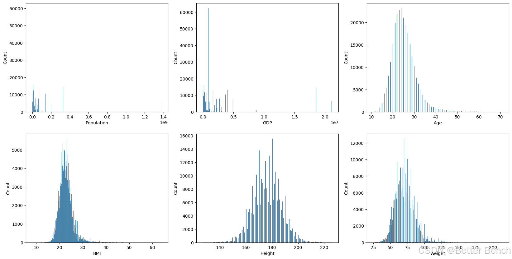
识别连续和离散数值特征中的偏度

在实现模型训练之前，需要了解的特征的分布，并将它们转换为正态分布，如果它们不限制偏差（即，这样模型就不会对具有较大值的变量更重要）。为此，首先测试了特征的偏度。

# Test for skewness in numerical variables: Population, GDP, Age BMI, Height, and Weight

def skewness():
    # Find skewness
    feature_names = ['Population', 'GDP', 'Age', 'BMI', 'Height', 'Weight']
    for i in range(len(feature_names)):
        print(f"{feature_names[i]} skew: {df_data[feature_names[i]].skew()}")
        
    # Create dist plots of each variable
    fig, axes = plt.subplots(ncols=3, nrows=2, figsize=(20, 10))
    for i, ax in zip(range(len(feature_names)), axes.flat):
        sns.histplot(df_data[feature_names[i]], ax=ax)
    plt.show()

skewness()

Population skew: 4.847316928926255
GDP skew: 2.8226162284359653
Age skew: 1.1319874071481901
BMI skew: 1.3722296331968096
Height skew: 0.007536973027835242
Weight skew: 0.7298782642302241

请添加图片描述

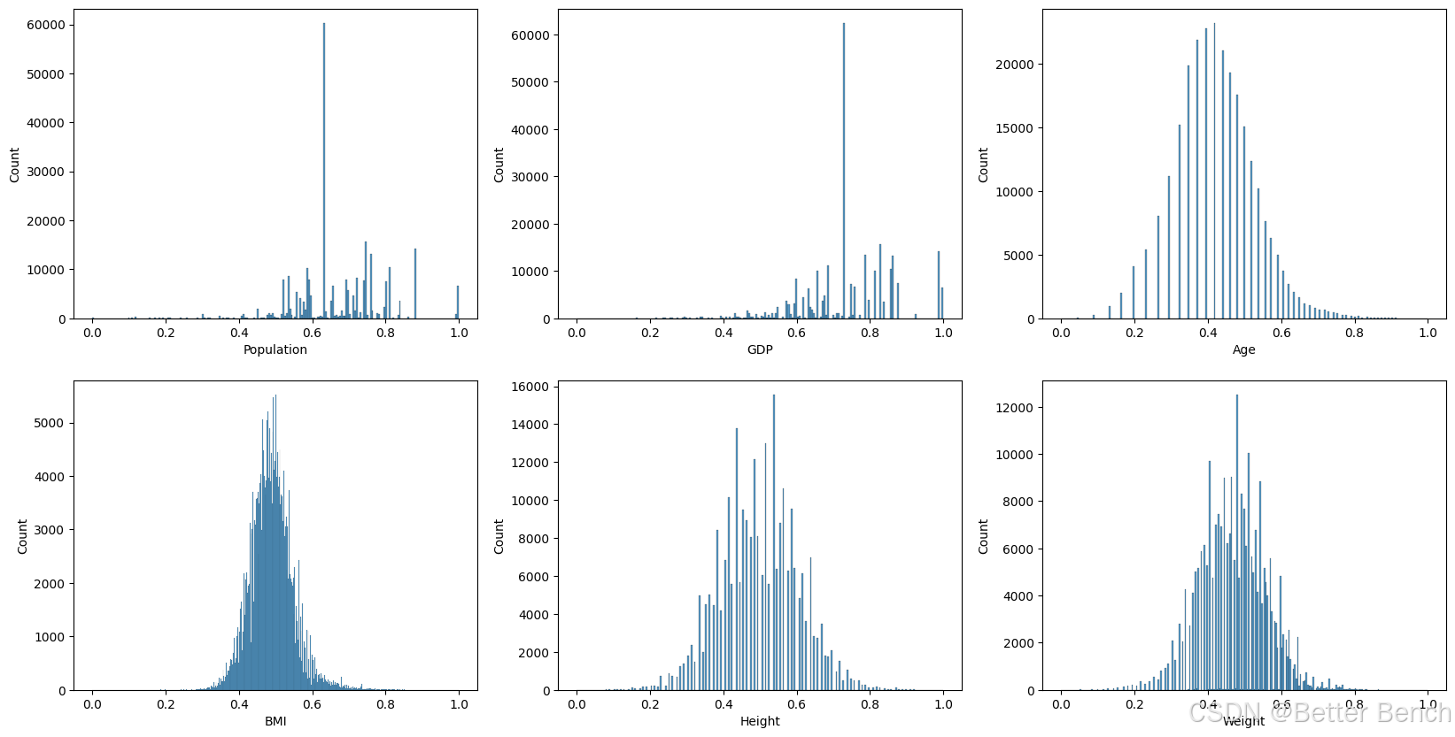
使用对数变换校正偏度

由于特征的分布通常是倾斜的，对每个特征应用一个对数函数来缩放和规范化它们，如下所示。

# Use log transformation to scale BMI, weight, age features
pop_log = np.log(df_data['Population'])
gdp_log = np.log(df_data['GDP'])
bmi_log = np.log(df_data['BMI'])
weight_log = np.log(df_data['Weight'])
age_log = np.log(df_data['Age'])

log_features = [pop_log, gdp_log, age_log, bmi_log, df_data['Height'], weight_log]
feature_names = ['Population', 'GDP', 'Age', 'BMI', 'Height', 'Weight']

# Normalize log transformed data
def normalize(column):
    upper = column.max()
    lower = column.min()
    y = (column-lower)/(upper-lower)
    return y

normal_features = []
for i in range(len(log_features)):
    norm = normalize(log_features[i])
    normal_features.append(norm)

# Empty dataframe with transformed and scaled values
cont_feature_sub_df = pd.DataFrame(columns = feature_names)

比较对数变换前后的偏度和分布

# Find and print new skewness
import scipy.stats

for i in range(len(normal_features)):
    print(f"{feature_names[i]} skew: {float(scipy.stats.skew(df_data[feature_names[i]]))}")
    print(f"{feature_names[i]} log-transformed skew: {float(scipy.stats.skew(normal_features[i]))} \n")
    # Add transformed values to dataframe
    cont_feature_sub_df[feature_names[i]] = normal_features[i]
    
# Create new dist plots with scaled and transformed variables
fig, axes = plt.subplots(ncols=3, nrows=2, figsize=(20, 10))
for i, ax in zip(range(len(normal_features)), axes.flat):
    sns.histplot(normal_features[i], ax=ax, label=feature_names[i])
plt.show()

Population skew: 4.847289663577969
Population log-transformed skew: -0.04977191246066552 

GDP skew: 2.822600351691021
GDP log-transformed skew: -0.42489600377264997 

Age skew: 1.1319810399080523
Age log-transformed skew: 0.23616538067882106 

BMI skew: 1.3722219146342678
BMI log-transformed skew: 0.5696356255853973 

Height skew: 0.007536930633620538
Height log-transformed skew: 0.007536930633621244 

Weight skew: 0.7298741587868682
Weight log-transformed skew: -0.03659542012833335

请添加图片描述

3.1.8 目标变量标签编码

因为的目标变量包含分类值（bronze, silver, gold, none），使用标签编码将的目标值转换为ML模型的数值，其中0代表金牌，1代表银牌，2代表铜牌，3代表没有奖牌。决定使用标签编码而不是单热编码来解释目标值中的不均匀权重，因为标签编码对更高的值更重要。例如，因为知道在现实生活中参加奥运会的运动员没有赢得奖牌的可能性更大，所以将最大值3赋给没有奖牌，这样这个值就更有分量了。

# Dictionary of numerical values corresponding to target categories
target_labels = {'Gold':0, 'Silver':1, 'Bronze':2, 'None':3}

# Use dictionary to transform each target value
def transform_medals(column):
    return target_labels[column]

# Apply transformation and create new dataframe with encoded target values
target_encoded_df = df_data
target_encoded_df["target"] = df_data["target"].apply(transform_medals)

3.1.9 用于模型测试的各种转换数据集

原始数据集与目标变量编码

这个数据集主要用于数据探索而不是训练

target_encoded_df

	Country	Population	GDP	Sex	Age	Height	Weight	Year	BMI	Season	Sport	Event	target
0	Indonesia	260580739	3028000.0	M	20.0	162.0	57.0	1956	21.719250	Summer	Athletics	Athletics Men's 100 metres	3
1	Indonesia	260580739	3028000.0	M	22.0	160.0	56.0	1960	21.875000	Summer	Weightlifting	Weightlifting Men's Bantamweight	3
2	Indonesia	260580739	3028000.0	M	37.0	172.0	70.0	1960	23.661439	Summer	Sailing	Sailing Mixed Three Person Keelboat	3
3	Indonesia	260580739	3028000.0	M	18.0	172.0	66.0	1960	22.309356	Summer	Cycling	Cycling Men's 100 kilometres Team Time Trial	3
4	Indonesia	260580739	3028000.0	M	18.0	172.0	66.0	1960	22.309356	Summer	Cycling	Cycling Men's Road Race, Individual	3
...	...	...	...	...	...	...	...	...	...	...	...	...	...
266670	New Zealand	4510327	174800.0	M	25.0	183.0	78.0	2016	23.291230	Summer	Hockey	Hockey Men's Hockey	3
266671	New Zealand	4510327	174800.0	F	18.0	159.0	58.0	2016	22.942130	Summer	Diving	Diving Women's Springboard	3
266672	New Zealand	4510327	174800.0	M	36.0	175.0	73.0	2016	23.836735	Summer	Shooting	Shooting Men's Small-Bore Rifle, Prone, 50 metres	3
266673	New Zealand	4510327	174800.0	M	32.0	189.0	70.0	2016	19.596316	Summer	Rowing	Rowing Men's Lightweight Coxless Fours	3
266674	New Zealand	4510327	174800.0	F	19.0	165.0	67.0	2016	24.609734	Summer	Rugby Sevens	Rugby Sevens Women's Rugby Sevens	1

266675 rows × 13 columns

没有日志转换或规范化的数据集

# Merge dataset without log transformation
non_transf_features = df_data[['Population', 'GDP', 'Age', 'BMI', 'Height', 'Weight']]
combined_df = pd.concat([cat_feature_sub_df, non_transf_features, bin_feature_sub_df, target_encoded_df['target']], axis=1)
combined_df

	Country	Year	Sport	Event	Population	GDP	Age	BMI	Height	Weight	Sex_F	Sex_M	Season_Summer	Season_Winter	target
0	77	13	3	30	260580739	3028000.0	20.0	21.719250	162.0	57.0	0.0	1.0	1.0	0.0	3
1	77	14	54	540	260580739	3028000.0	22.0	21.875000	160.0	56.0	0.0	1.0	1.0	0.0	3
2	77	14	36	381	260580739	3028000.0	37.0	23.661439	172.0	70.0	0.0	1.0	1.0	0.0	3
3	77	14	14	201	260580739	3028000.0	18.0	22.309356	172.0	66.0	0.0	1.0	1.0	0.0	3
4	77	14	14	214	260580739	3028000.0	18.0	22.309356	172.0	66.0	0.0	1.0	1.0	0.0	3
...	...	...	...	...	...	...	...	...	...	...	...	...	...	...	...
266670	123	34	24	310	4510327	174800.0	25.0	23.291230	183.0	78.0	0.0	1.0	1.0	0.0	3
266671	123	34	15	239	4510327	174800.0	18.0	22.942130	159.0	58.0	1.0	0.0	1.0	0.0	3
266672	123	34	37	404	4510327	174800.0	36.0	23.836735	175.0	73.0	0.0	1.0	1.0	0.0	3
266673	123	34	33	352	4510327	174800.0	32.0	19.596316	189.0	70.0	0.0	1.0	1.0	0.0	3
266674	123	34	35	367	4510327	174800.0	19.0	24.609734	165.0	67.0	1.0	0.0	1.0	0.0	1

266675 rows × 15 columns

具有日志转换和规范化的数据集

# Merge dataset with log transformation
df_log_transf = pd.concat([cat_feature_sub_df, cont_feature_sub_df, bin_feature_sub_df, target_encoded_df['target']], axis=1)
df_log_transf

	Country	Year	Sport	Event	Population	GDP	Age	BMI	Height	Weight	Sex_F	Sex_M	Season_Summer	Season_Winter	target
0	77	13	3	30	0.860060	0.836021	0.320593	0.469387	0.353535	0.383855	0.0	1.0	1.0	0.0	3
1	77	14	54	540	0.860060	0.836021	0.371704	0.472901	0.333333	0.375612	0.0	1.0	1.0	0.0	3
2	77	14	36	381	0.860060	0.836021	0.650489	0.511500	0.454545	0.479540	0.0	1.0	1.0	0.0	3
3	77	14	14	201	0.860060	0.836021	0.264093	0.482568	0.454545	0.452135	0.0	1.0	1.0	0.0	3
4	77	14	14	214	0.860060	0.836021	0.264093	0.482568	0.454545	0.452135	0.0	1.0	1.0	0.0	3
...	...	...	...	...	...	...	...	...	...	...	...	...	...	...	...
266670	123	34	24	310	0.519408	0.595360	0.440255	0.503746	0.565657	0.529939	0.0	1.0	1.0	0.0	3
266671	123	34	15	239	0.519408	0.595360	0.264093	0.496320	0.323232	0.391955	1.0	0.0	1.0	0.0	3
266672	123	34	37	404	0.519408	0.595360	0.635797	0.515129	0.484848	0.499084	0.0	1.0	1.0	0.0	3
266673	123	34	33	352	0.519408	0.595360	0.572635	0.418813	0.626263	0.479540	0.0	1.0	1.0	0.0	3
266674	123	34	35	367	0.519408	0.595360	0.293087	0.530821	0.383838	0.459139	1.0	0.0	1.0	0.0	1

266675 rows × 15 columns

3.2. 数据探索

3.2.1 数据集初步探索

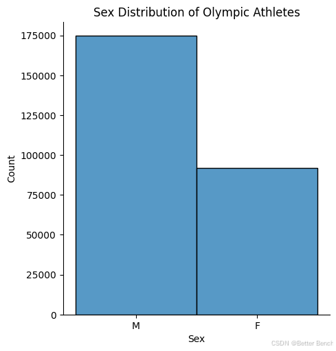
下面的可视化展示了对数据集的初步探索。下面的图表显示了的样本按性别分布。该分布图表明，的数据样本中男性运动员明显多于女性运动员，男性运动员的数量（14万+）大约是女性运动员数量（7万+）的两倍。

sns.displot(target_encoded_df, x="Sex")

#specify the title
title = "Sex Distribution of Olympic Athletes"

#set the title of the plot
plt.title(title)

Text(0.5, 1.0, 'Sex Distribution of Olympic Athletes')

请添加图片描述

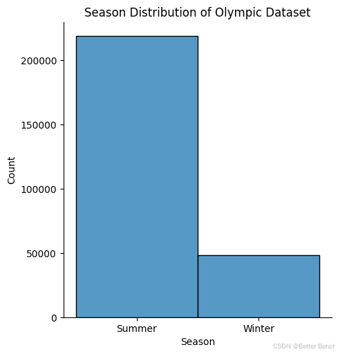
下面的图表显示了的样本在奥运会季节的分布。该分布图表明，的数据样本中夏季运动员的数量明显多于冬季运动员，夏季运动员的数量（175,000+）是冬季运动员数量（40,000+）的三倍。这是有道理的，因为夏季奥运会的项目和项目也比冬季奥运会多，所以总的来说，参加夏季奥运会的运动员要比冬季奥运会多。

sns.displot(target_encoded_df, x="Season")

#specify the title
title = "Season Distribution of Olympic Dataset"

#set the title of the plot
plt.title(title)

Text(0.5, 1.0, 'Season Distribution of Olympic Dataset')

请添加图片描述

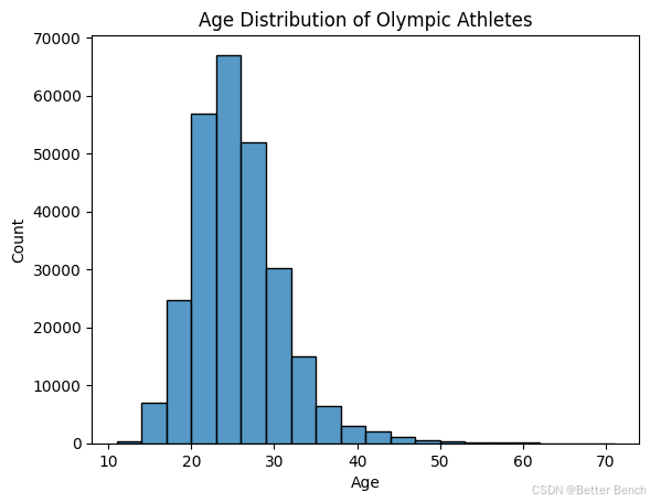
下面的直方图显示了的样本按年龄分布。直方图显示，年龄分布呈正偏态，样本中大多数运动员集中在20-30岁左右，年龄越大，运动员数量向右急剧减少。这是有道理的，因为奥运会选手必须保持强壮和最佳的健康状态才能参加艰苦的训练和比赛，而年轻的年龄范围（20-30岁）通常是人们处于最佳健康状态的时候。

sns.histplot(target_encoded_df, x="Age", bins=20)

#specify the title
title = "Age Distribution of Olympic Athletes"

#set the title of the plot
plt.title(title)

Text(0.5, 1.0, 'Age Distribution of Olympic Athletes')

请添加图片描述

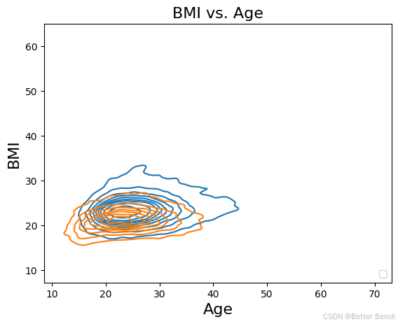
下面的核密度图显示了运动员在年龄和BMI方面的分布。如图所示，“最密集”的区域由最小的内圈表示，这表明大多数女运动员（橙色表示）聚集在20岁出头（年龄），体重指数约为21。同样，大量男性运动员的身体质量指数在25左右，年龄在20岁出头。女性运动员的圆形更密集（紧密地聚集在一起），说明女性的年龄和bmi分布相对较小。相比之下，男性运动员的图密度较低（有更多的形状，分组距离更远），表明年龄/ bmi的分布更分散。

# Create and display the kernel density plot
graph = sns.kdeplot(x="Age", y="BMI", hue = "Sex", 
                        data = df_data)

# Specify the title
title = "BMI vs. Age"

# Set the title of the plot
graph.set_title(title, size = 16)

# Add labels to the axes  
graph.set_xlabel("Age", size = 16)
graph.set_ylabel("BMI", size = 16)

# Move the legend to lower right
plt.legend(loc="lower right")

<matplotlib.legend.Legend at 0x1a017f8af10>

请添加图片描述

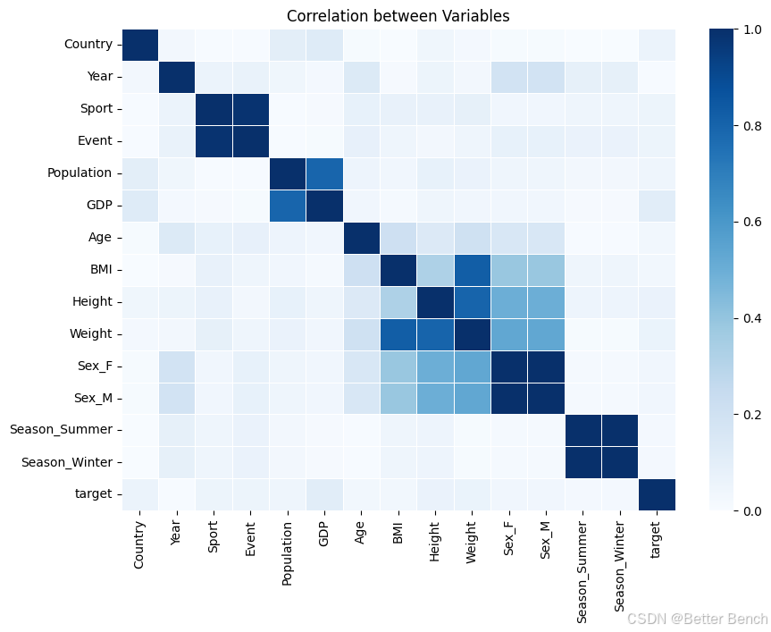
def heatmap(dataframe, start_col, end_col, color):
    df_features = dataframe.iloc[:, start_col:end_col]
    
    # Find the correlation coefficient between each trait as a new dataframe (absolute value applied so all coefficients between 0 and 1)
    df_corr = df_features.corr().abs()
    
    # Set sizes of figure
    fig_dims = (10, 7)
    fig, ax = plt.subplots(figsize=fig_dims)
    
    # Create a blue heatmap of strengh of correlation
    viz = sns.heatmap(df_corr, vmin=0, vmax=1, linewidths=0.5, cmap=color, ax=ax)
    viz.set(title="Correlation between Variables")

3.2.2 数据探索按国家和奖牌总数排序

创建新的数据df，按国家和奖牌总数排序

为了从更简洁的角度更好地理解和可视化的数据，决定创建另一个数据框架，将原始数据框架按国家分组，并查看每个国家获得的总奖牌、每个国家派出的运动员总数、每个国家运动员的年龄、体重、身高、BMI中位数以及每个国家最常见的运动、项目和季节等指标。能够将这些计算出的指标与其他列（如每个国家的GDP和人口）进行比较，以更好地了解这些变量如何相互影响。

# Function used to change medal type to number of medals (to sum by country after)
def change_target(medal):
    if medal == 0 or medal == 1 or medal == 2:
        medal = 1
    else:
        medal = 0
    return medal

# Count number of entries for each country to determine number of athletes and add to df_data
df_data['Number of Athletes'] = df_data.groupby('Country')['Country'].transform('count') 
df_data

	Country	Population	GDP	Sex	Age	Height	Weight	Year	BMI	Season	Sport	Event	target	Number of Athletes
0	Indonesia	260580739	3028000.0	M	20.0	162.0	57.0	1956	21.719250	Summer	Athletics	Athletics Men's 100 metres	3	334
1	Indonesia	260580739	3028000.0	M	22.0	160.0	56.0	1960	21.875000	Summer	Weightlifting	Weightlifting Men's Bantamweight	3	334
2	Indonesia	260580739	3028000.0	M	37.0	172.0	70.0	1960	23.661439	Summer	Sailing	Sailing Mixed Three Person Keelboat	3	334
3	Indonesia	260580739	3028000.0	M	18.0	172.0	66.0	1960	22.309356	Summer	Cycling	Cycling Men's 100 kilometres Team Time Trial	3	334
4	Indonesia	260580739	3028000.0	M	18.0	172.0	66.0	1960	22.309356	Summer	Cycling	Cycling Men's Road Race, Individual	3	334
...	...	...	...	...	...	...	...	...	...	...	...	...	...	...
266670	New Zealand	4510327	174800.0	M	25.0	183.0	78.0	2016	23.291230	Summer	Hockey	Hockey Men's Hockey	3	7760
266671	New Zealand	4510327	174800.0	F	18.0	159.0	58.0	2016	22.942130	Summer	Diving	Diving Women's Springboard	3	7760
266672	New Zealand	4510327	174800.0	M	36.0	175.0	73.0	2016	23.836735	Summer	Shooting	Shooting Men's Small-Bore Rifle, Prone, 50 metres	3	7760
266673	New Zealand	4510327	174800.0	M	32.0	189.0	70.0	2016	19.596316	Summer	Rowing	Rowing Men's Lightweight Coxless Fours	3	7760
266674	New Zealand	4510327	174800.0	F	19.0	165.0	67.0	2016	24.609734	Summer	Rugby Sevens	Rugby Sevens Women's Rugby Sevens	1	7760

266675 rows × 14 columns

# Create df_summary grouped by country
df_summary = df_data.iloc[:, 0:14]
df_summary['GDP per Capita'] = df_summary['GDP']/df_summary['Population']

# Find total medals, median BMI, median Age, median Weight, most common event, most common sport, most common season, year with most athletes, number of athletes, GDP, GDP per capita, and Population for each country
df_summary['Total Medals'] = df_summary['target'].apply(change_target)
df_summary = df_summary.groupby('Country', as_index=False).agg({'Total Medals': 'sum', 'Population':lambda x: pd.Series.mode(x)[0],
                                                                'GDP':lambda x: pd.Series.mode(x)[0], 'Age': 'median', 'Height':'median','Weight':'median', 'Year':lambda x: pd.Series.mode(x)[0],
                                                                'BMI':'median', 'Season':lambda x: pd.Series.mode(x)[0], 'Sport':lambda x: pd.Series.mode(x)[0], 
                                                                'GDP per Capita':lambda x: pd.Series.mode(x)[0], 'Event':lambda x: pd.Series.mode(x)[0], 'Number of Athletes':lambda x: pd.Series.mode(x)[0]})
df_summary['Medals per Athlete'] = (df_summary['Total Medals']/df_summary['Number of Athletes'])
df_summary

	Country	Total Medals	Population	GDP	Age	Height	Weight	Year	BMI	Season	Sport	GDP per Capita	Event	Number of Athletes	Medals per Athlete
0	Afghanistan	2	34124811	64080.0	23.0	170.0	64.0	1960	22.128136	Summer	Wrestling	0.001878	Athletics Men's 100 metres	54	0.037037
1	Albania	0	3047987	33900.0	23.0	170.0	69.0	2008	23.087868	Summer	Weightlifting	0.011122	Shooting Women's Sporting Pistol, 25 metres	57	0.000000
2	Algeria	15	40969443	609400.0	24.0	175.0	66.0	2016	21.971336	Summer	Athletics	0.014875	Handball Men's Handball	481	0.031185
3	American Samoa	0	51504	711.0	26.0	175.0	82.0	1988	26.595745	Summer	Athletics	0.013805	Athletics Men's 100 metres	21	0.000000
4	Andorra	0	85702	3327.0	22.0	173.0	71.0	2010	23.255019	Winter	Alpine Skiing	0.038821	Alpine Skiing Men's Giant Slalom	135	0.000000
...	...	...	...	...	...	...	...	...	...	...	...	...	...	...	...
184	Venezuela	15	31304016	468600.0	24.0	173.0	69.0	2008	22.720438	Summer	Swimming	0.014969	Cycling Men's Road Race, Individual	785	0.019108
185	Vietnam	4	96160163	594900.0	23.0	165.0	58.0	1980	20.831262	Summer	Swimming	0.006187	Cycling Men's Road Race, Individual	182	0.021978
186	Yemen	0	28036829	73450.0	21.0	168.0	61.0	1988	21.773842	Summer	Athletics	0.002620	Athletics Men's 1,500 metres	37	0.000000
187	Zambia	1	15972000	65170.0	23.0	175.0	67.0	1988	21.604938	Summer	Athletics	0.004080	Football Men's Football	128	0.007812
188	Zimbabwe	22	13805084	28330.0	24.0	175.0	66.0	1980	22.545959	Summer	Athletics	0.002052	Football Women's Football	299	0.073579

189 rows × 15 columns

从df_summary中创建包含前20个获奖国家的新数据框架

# Create df of top 20 countries with most medals
top_df = df_summary.nlargest(n=20, columns='Total Medals', keep='first')
top_df

	Country	Total Medals	Population	GDP	Age	Height	Weight	Year	BMI	Season	Sport	GDP per Capita	Event	Number of Athletes	Medals per Athlete
122	Netherlands	11328	17084719	870800.0	25.0	180.0	73.0	2016	22.460034	Summer	Swimming	0.050970	Hockey Men's Hockey	59664	0.189863
177	USA	4383	326625791	18560000.0	24.0	178.0	72.0	1992	22.720438	Summer	Athletics	0.056823	Ice Hockey Men's Ice Hockey	14214	0.308358
143	Russia	3610	142257519	3745000.0	25.0	176.0	70.0	1988	22.720438	Summer	Athletics	0.026325	Ice Hockey Men's Ice Hockey	10398	0.347182
63	Germany	3189	80594017	3979000.0	24.0	178.0	70.0	1972	22.530864	Summer	Athletics	0.049371	Ice Hockey Men's Ice Hockey	13183	0.241902
9	Australia	1210	23232413	1189000.0	24.0	177.0	71.0	2000	22.662709	Summer	Swimming	0.051178	Hockey Men's Hockey	6630	0.182504
31	Canada	1060	35623680	1674000.0	24.0	175.0	70.0	1988	22.656250	Summer	Athletics	0.046991	Ice Hockey Men's Ice Hockey	7966	0.133066
82	Italy	1060	62137802	2221000.0	25.0	175.0	70.0	1992	22.675737	Summer	Athletics	0.035743	Water Polo Men's Water Polo	7697	0.137716
37	China	1038	1379302771	21140000.0	23.0	172.0	65.0	2008	21.913806	Summer	Swimming	0.015327	Basketball Men's Basketball	6555	0.158352
176	UK	1031	64769452	2788000.0	25.0	175.0	70.0	2012	22.530864	Summer	Athletics	0.043045	Hockey Men's Hockey	7766	0.132758
60	France	987	67106161	2699000.0	25.0	175.0	69.0	1992	22.275310	Summer	Athletics	0.040220	Ice Hockey Men's Ice Hockey	7977	0.123731
123	New Zealand	844	4510327	174800.0	25.0	178.0	73.0	2016	22.985398	Summer	Hockey	0.038756	Hockey Men's Hockey	7760	0.108763
85	Japan	843	126451398	4932000.0	24.0	168.0	62.0	1964	22.038567	Summer	Gymnastics	0.039003	Volleyball Women's Volleyball	7487	0.112595
74	Hungary	791	9850845	267600.0	24.0	176.0	70.0	1992	22.598140	Summer	Gymnastics	0.027165	Water Polo Men's Water Polo	4681	0.168981
164	Sweden	765	9960487	498100.0	25.0	179.0	72.0	1988	22.720438	Summer	Athletics	0.050008	Ice Hockey Men's Ice Hockey	5314	0.143959
59	Finland	724	5491218	224137.0	25.0	176.0	70.0	1952	22.516126	Summer	Athletics	0.040817	Ice Hockey Men's Ice Hockey	4389	0.164958
142	Romania	597	21529967	441000.0	24.0	173.0	67.0	1980	22.491349	Summer	Gymnastics	0.020483	Rowing Women's Coxed Eights	3477	0.171700
158	South Korea	561	51181299	1929000.0	23.0	172.0	65.0	1988	22.145329	Summer	Gymnastics	0.037690	Football Men's Football	3854	0.145563
138	Poland	548	38476269	1052000.0	25.0	175.0	70.0	1972	22.790358	Summer	Athletics	0.027342	Ice Hockey Men's Ice Hockey	5728	0.095670
45	Czech Republic	519	10674723	350900.0	25.0	176.0	71.0	1980	22.720438	Summer	Gymnastics	0.032872	Ice Hockey Men's Ice Hockey	4583	0.113245
128	Norway	514	5320045	364700.0	25.0	179.0	73.0	1972	22.545959	Winter	Cross Country Skiing	0.068552	Ice Hockey Men's Ice Hockey	3061	0.167919

从df_summary中创建包含每个运动员获得奖牌前20名的国家的新数据框

# Create df with top 20 countries with largest medals per athlete ratio
medal_per_athlete_df = df_summary.nlargest(n=20, columns='Medals per Athlete', keep='first')
medal_per_athlete_df.reset_index(inplace=True)
medal_per_athlete_df

	index	Country	Total Medals	Population	GDP	Age	Height	Weight	Year	BMI	Season	Sport	GDP per Capita	Event	Number of Athletes	Medals per Athlete
0	143	Russia	3610	142257519	3745000.0	25.0	176.0	70.0	1988	22.720438	Summer	Athletics	0.026325	Ice Hockey Men's Ice Hockey	10398	0.347182
1	177	USA	4383	326625791	18560000.0	24.0	178.0	72.0	1992	22.720438	Summer	Athletics	0.056823	Ice Hockey Men's Ice Hockey	14214	0.308358
2	130	Pakistan	107	204924861	988200.0	25.0	174.0	70.0	1960	22.592987	Summer	Hockey	0.004822	Hockey Men's Hockey	366	0.292350
3	63	Germany	3189	80594017	3979000.0	24.0	178.0	70.0	1972	22.530864	Summer	Athletics	0.049371	Ice Hockey Men's Ice Hockey	13183	0.241902
4	150	Serbia	467	7111024	101800.0	24.0	180.0	75.0	1984	23.405654	Summer	Athletics	0.014316	Water Polo Men's Water Polo	2342	0.199402
5	84	Jamaica	154	2990561	25390.0	24.0	176.0	68.0	2016	21.877551	Summer	Athletics	0.008490	Athletics Men's 4 x 400 metres Relay	809	0.190358
6	122	Netherlands	11328	17084719	870800.0	25.0	180.0	73.0	2016	22.460034	Summer	Swimming	0.050970	Hockey Men's Hockey	59664	0.189863
7	9	Australia	1210	23232413	1189000.0	24.0	177.0	71.0	2000	22.662709	Summer	Swimming	0.051178	Hockey Men's Hockey	6630	0.182504
8	43	Cuba	394	11147407	132900.0	24.0	175.0	72.0	1980	23.306680	Summer	Athletics	0.011922	Baseball Men's Baseball	2210	0.178281
9	142	Romania	597	21529967	441000.0	24.0	173.0	67.0	1980	22.491349	Summer	Gymnastics	0.020483	Rowing Women's Coxed Eights	3477	0.171700
10	74	Hungary	791	9850845	267600.0	24.0	176.0	70.0	1992	22.598140	Summer	Gymnastics	0.027165	Water Polo Men's Water Polo	4681	0.168981
11	135	Paraguay	17	6943739	64670.0	22.0	177.0	74.0	2004	23.355637	Summer	Football	0.009313	Football Men's Football	101	0.168317
12	128	Norway	514	5320045	364700.0	25.0	179.0	73.0	1972	22.545959	Winter	Cross Country Skiing	0.068552	Ice Hockey Men's Ice Hockey	3061	0.167919
13	11	Azerbaijan	44	9961396	167900.0	24.0	171.0	67.0	2016	22.832879	Summer	Wrestling	0.016855	Rhythmic Gymnastics Women's Group	263	0.167300
14	42	Croatia	139	4292095	94240.0	25.0	183.0	82.0	2008	24.092971	Summer	Swimming	0.021957	Water Polo Men's Water Polo	835	0.166467
15	59	Finland	724	5491218	224137.0	25.0	176.0	70.0	1952	22.516126	Summer	Athletics	0.040817	Ice Hockey Men's Ice Hockey	4389	0.164958
16	37	China	1038	1379302771	21140000.0	23.0	172.0	65.0	2008	21.913806	Summer	Swimming	0.015327	Basketball Men's Basketball	6555	0.158352
17	57	Ethiopia	53	105350020	174700.0	24.0	170.0	57.0	1980	19.265306	Summer	Athletics	0.001658	Athletics Men's Marathon	347	0.152738
18	47	Denmark	255	5605948	264800.0	25.0	180.0	73.0	1972	22.448015	Summer	Swimming	0.047236	Handball Men's Handball	1704	0.149648
19	115	Montenegro	14	642550	10610.0	27.0	185.0	86.0	2016	24.569314	Summer	Water Polo	0.016512	Water Polo Men's Water Polo	94	0.148936

按国家分组的数据框可视化

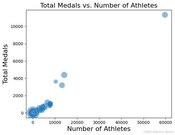
下面的散点图显示，运动员人数与获得的奖牌总数之间存在较强的正相关关系；换句话说，一个国家派出越多的运动员参加奥运会，这个国家就越有可能赢得更多的奖牌。这是有道理的，因为有更多的运动员参加比赛，自然意味着一个国家有更多的参与者，就更有可能赢得更多的奖牌。虽然每个点的大小代表人均GDP，但人均GDP与运动员数量/总奖牌数之间似乎没有很强的相关性；大多数获得奖牌最多的国家的人均国内生产总值既不太大也不太小。为了解释这种差异，并创建一个使各国之间具有可比性的指标，创建了“运动员人均奖牌数”这一列，通过将一个国家的总奖牌数除以该国的运动员总数来计算。

# Create and display the scatterplot
graph = sns.scatterplot(x="Number of Athletes", y="Total Medals", size = "GDP per Capita", sizes= (10, 1000), data = df_summary, alpha=.5, legend=False)

# Specify the title
title = "Total Medals vs. Number of Athletes"

# Set the title of the plot
graph.set_title(title, size = 16)

# Add labels to the axes  
graph.set_xlabel("Number of Athletes", size = 16)
graph.set_ylabel("Total Medals", size = 16)

Text(0, 0.5, 'Total Medals')

请添加图片描述

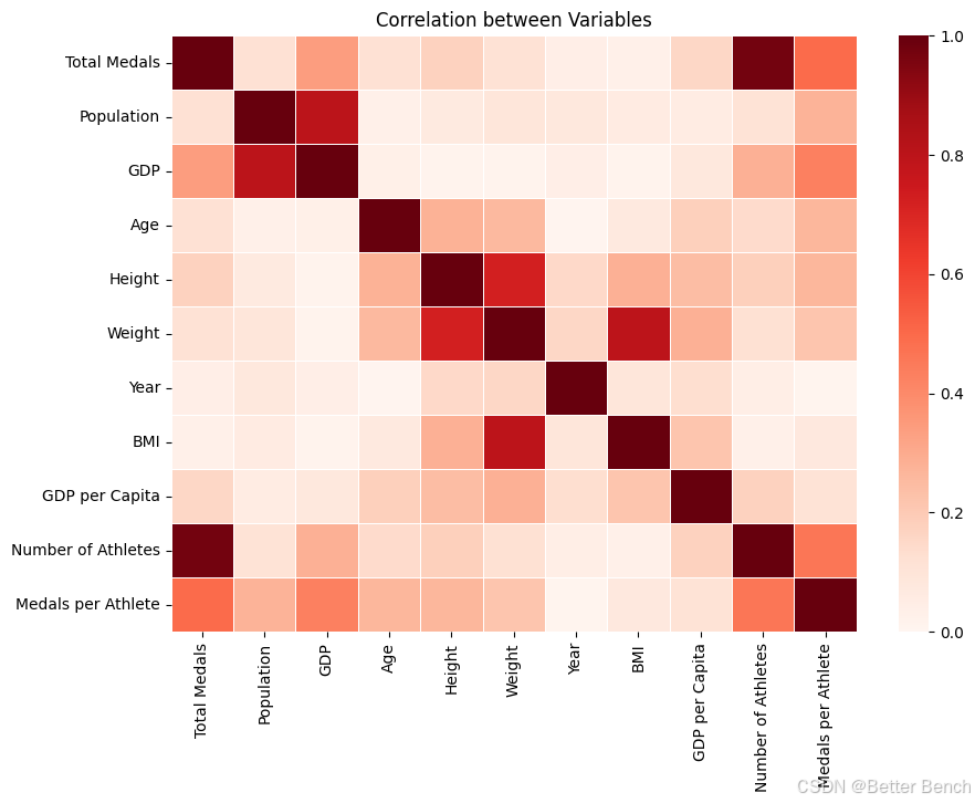
描绘各国特征之间相关性的热图（与运动员人均奖牌数相比较的特征）

下面的热图显示了按国家分组的数据框中每个变量之间的相关性有多强。从热图中可以看出，GDP与总奖牌数、运动员人数与总奖牌数、GDP与参加奥运会的运动员人数等变量之间存在着中等到强的相关性(这些变量之间不是由彼此推导出来的（例如，BMI是由体重和身高计算出来的）。此外，国内生产总值与运动员人均奖牌数有适度的相关性，这表明国内生产总值较高（较富裕）的国家更有可能赢得更多的奖牌。

heatmap(df_summary, 0, 16, 'Reds')

请添加图片描述

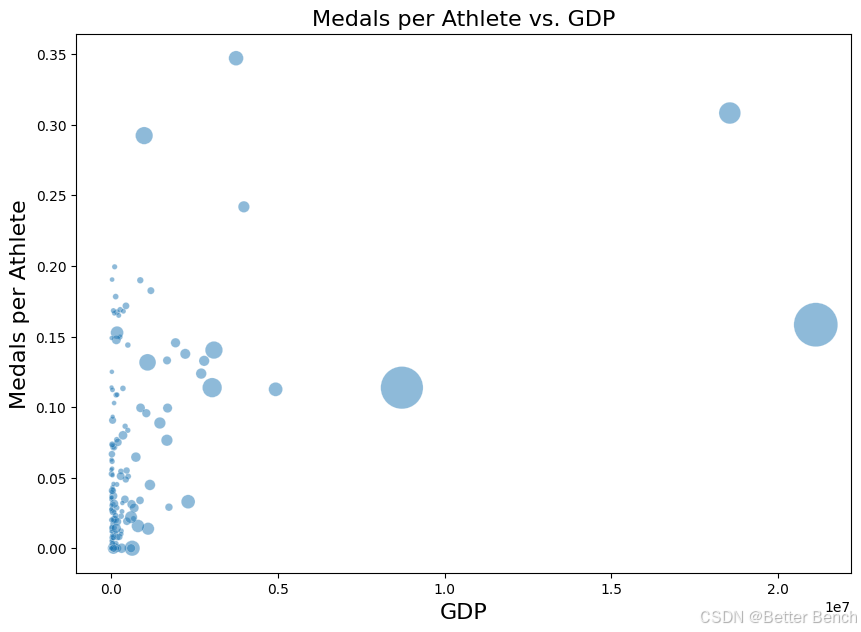
下面的散点图比较了一个国家的GDP和每个运动员的奖牌数。散点图的总体趋势显示出轻微的正相关，这意味着一个国家的GDP越高，该国每位运动员获得的奖牌就越多。然而，图表中也有许多数据点代表了GDP值较低但运动员人均奖牌数较高的国家，这就是为什么正相关性不那么强的原因。

# Set sizes of figure
fig_dims = (10, 7)
fig, ax = plt.subplots(figsize=fig_dims)

# Create and display the scatterplot
graph = sns.scatterplot(x="GDP", y="Medals per Athlete", size = "Population", sizes= (10, 1000), data = df_summary, alpha=.5, ax=ax, legend=False)

# Specify the title
title = "Medals per Athlete vs. GDP"

# Set the title of the plot
graph.set_title(title, size = 16)

# Add labels to the axes  
graph.set_xlabel("GDP", size = 16)
graph.set_ylabel("Medals per Athlete", size = 16)

Text(0, 0.5, 'Medals per Athlete')

请添加图片描述

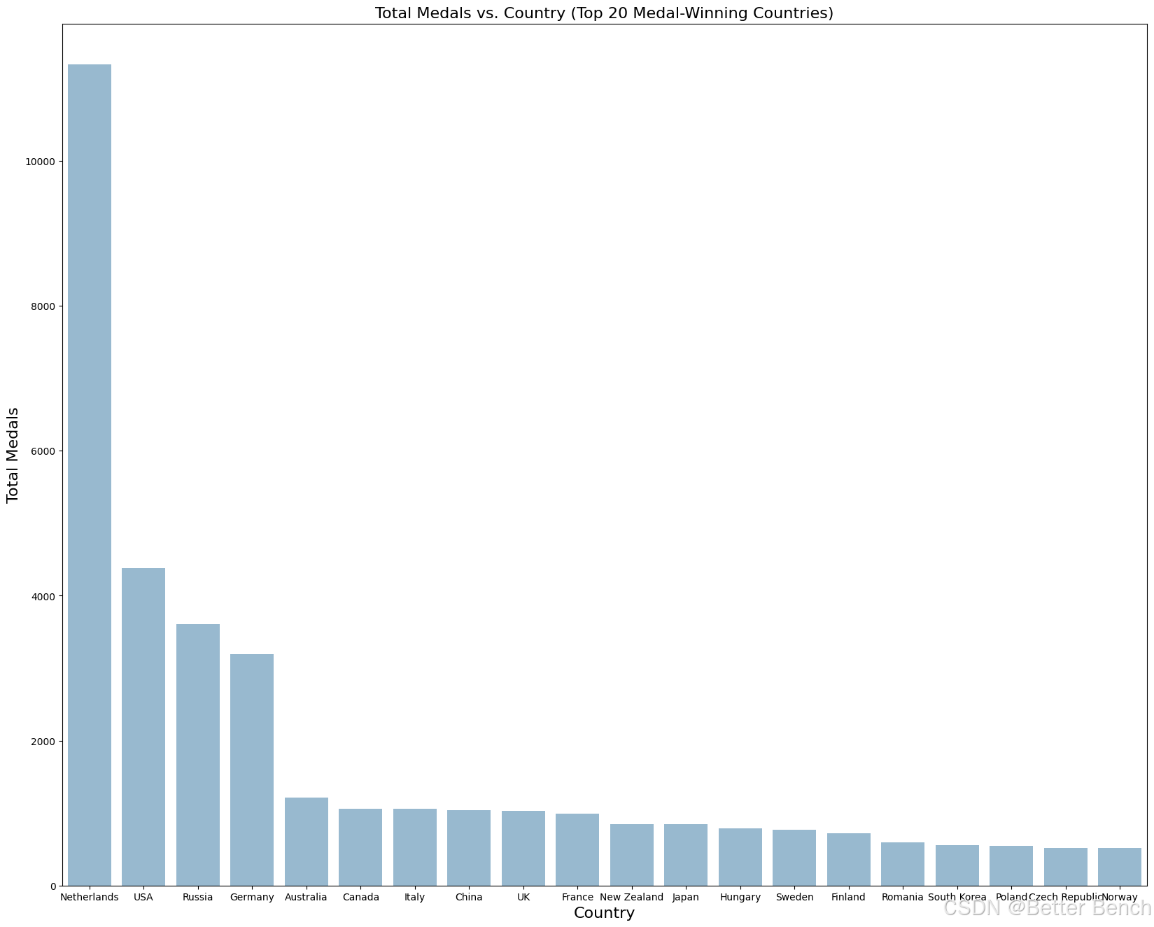
下面的条形图展示了获得奥运会奖牌最多的前20个国家以及每个国家获得的奖牌总数。从图中可以看出，总的来说，美国的奖牌数最多，达到4000 +枚，其次是俄罗斯（3500 +枚），然后是德国（3000 +枚）。

# Set sizes of figure
fig_dims = (20, 16)
fig, ax = plt.subplots(figsize=fig_dims)

# Create and display the bar plot
graph = sns.barplot(x="Country", y="Total Medals", data = top_df, alpha=.5, ax=ax)

# Specify the title
title = "Total Medals vs. Country (Top 20 Medal-Winning Countries)"

# Set the title of the plot
graph.set_title(title, size = 16)

# Add labels to the axes  
graph.set_xlabel("Country", size = 16)
graph.set_ylabel("Total Medals", size = 16)

Text(0, 0.5, 'Total Medals')

请添加图片描述

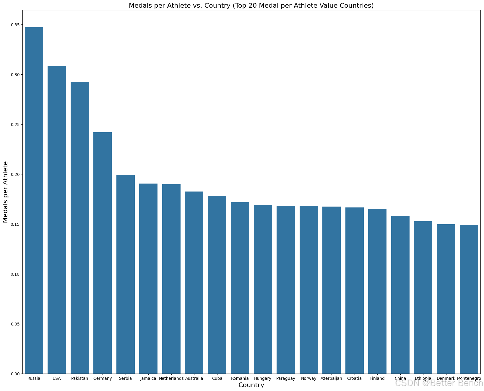
为了将奖牌总数和运动员数量这两个指标放在一起，使每个国家获得的奖牌数量更具可比性（因为已经展示了参加奥运会的运动员数量与获得的奖牌总数直接相关），下面的条形图显示了奖牌数量排名前20的国家和每个国家每位运动员的奖牌数量。从图表中可以明显看出，总体而言，俄罗斯的人均奖牌数最高，约为0.34枚，美国以0.31枚紧随其后，巴基斯坦以0.29枚紧随其后。

# Set sizes of figure
fig_dims = (20, 16)
fig, ax = plt.subplots(figsize=fig_dims)

# Create and display the bar plot
graph = sns.barplot(x="Country", y="Medals per Athlete", data = medal_per_athlete_df, ax=ax)

# Specify the title
title = "Medals per Athlete vs. Country (Top 20 Medal per Athlete Value Countries)"

# Set the title of the plot
graph.set_title(title, size = 16)

# Add labels to the axes  
graph.set_xlabel("Country", size = 16)
graph.set_ylabel("Medals per Athlete", size = 16)

Text(0, 0.5, 'Medals per Athlete')

请添加图片描述

3.3. Model Training

3.3.1 模型训练方法概述

算法:

kNN Classifier
Decision Tree
Naive Bayes

抽样方法:

Simple Random Sampling
SMOTE Sampling

数据转换方法:

Log-transformations (see data wrangling)
Standard Scaler
Minmax Scaler

评估指标:

Accuracy
Precision
Recall
F1-score

3.3.2 将训练模型定义为字典

# Import models: KNN, Naive Bayse, Decision Tree
from sklearn.neighbors import KNeighborsClassifier
from sklearn.naive_bayes import GaussianNB
from sklearn.tree import DecisionTreeClassifier
from sklearn.model_selection import train_test_split

# Store estimators as a dictionary for easy reference when training and testing
estimators = {'k-Nearest Neighbor': KNeighborsClassifier(), 'Gaussian Naive Bayes': GaussianNB(), 
              'Decision Tree': DecisionTreeClassifier()}

3.3.3 初始化评估度量数据框架

使用这个数据框架来存储不同的建模技术。这包括各种缩放方法、采样方法和超参数调优。对于性能指标，使用准确性、f1-score、召回率和精度。为不同的模型和优化技术找到了这些值。

在模型训练中，使用一种称为score的精度度量，它可以在sklearn库中以.score（）的形式获得。这通常用于确定模型准确性，因为它比较了训练集或测试集上的预测输出与实际输出之间的差异。本质上，特征被输入到模型中，并被训练来预测输出，即目标变量；然后将该预测输出与实际目标变量进行比较，并计算百分比精度。

除了准确性之外，还使用一些不同的常见分类性能评估指标：精度、召回率和f1-score。使用sk-learn的分类报告功能找到了所有这些。

精确度测量tp / (tp + fp)的比率，或真阳性率。通常，这个评估指标用于分类模型，因为它确定了给定模型不标记假阳性的能力。在项目的应用中，如果一名运动员被认定为奖牌获得者，但实际上并没有赢得比赛。这是衡量模型能力的一个重要指标，因为它很好地衡量了模型回答的问题的能力：能预测谁会赢吗？如果的准确率很低，可能会把失败者误认为是赢家。

回忆通常被理解为精确的反义词。它测量的是真负率，或tp / (tp + fn)。在项目的上下文中，选择了这个评估指标，因为它确定了能够正确识别奥运奖牌获得者的频率。

F1-score是准确率和召回率之间的加权平均值，计算公式为F1 = 2 （准确率召回率）/（准确率+召回率）。认为这个分数对于评估的模型性能很重要，因为它在某种意义上是“两全其美”。精准度可能高估了准确预测的奖牌预测指标的数量，而不是意外地将其归类为“无”，召回率过于依赖于不过度分配奖牌获得者，f1分数给了一个很好的中间点。

# Different forms of the three models to test
parameters = ['Base', 'Random Sampling', 'SMOTE Sampling', 'Min Max Scaler', 'Standard Scaler', 'Min Max Scaler (Log)', 'Standard Scaler (Log)', 'Feature Selection', 'Grid Search CV']

# Empty lists to add estimator models and model selection types as column labels
methods = []
models = []

# Add to column names using estimators dictionary
for parameter in parameters:
    for key, value in estimators.items():
        methods.append(parameter)
        models.append(key)

# Different performance metrics from classification report 

# Performance metrics for each target value (0: Gold, 1: Silver, 2: Bronze, 3: None)
report_keys = ['0', '1', '2', '3']

# Different metrics and grouping functions
report_agg = ['macro avg', 'weighted avg']
report_values = ['precision', 'recall', 'f1-score', 'support']

# Initialize empty lists to add metric names
column_idx = []
column_metric = []

# Add to list of row names
# For performance metrics based off of target value (0, 1, 2, 3)
for key in report_keys:
    for value in report_values:
        column_idx.append(key)
        column_metric.append(value)

# For accuracy performance metric
column_idx.append('all')
column_metric.append('accuracy')

# For aggregate performance metrics
for agg in report_agg:
    for value in report_values:
        column_idx.append(agg)
        column_metric.append(value)

使用预定义的列和行初始化评估指标的空数据集

# Define columns and rows (indices) for empty dataframe
columns = [methods, models]
indices = [column_idx, column_metric]

# Fill dataframe with 0 values (to be replaced with actual performance metric values)
data = [ [0] * len(methods) for _ in range(len(column_idx))]

# Create dataframe to store evaluation metrics
performance = pd.DataFrame(data, columns = columns, index = indices)
performance

		Base			Random Sampling			SMOTE Sampling			Min Max Scaler	...	Min Max Scaler (Log)	Standard Scaler (Log)			Feature Selection			Grid Search CV
		k-Nearest Neighbor	Gaussian Naive Bayes	Decision Tree	k-Nearest Neighbor	Gaussian Naive Bayes	Decision Tree	k-Nearest Neighbor	Gaussian Naive Bayes	Decision Tree	k-Nearest Neighbor	...	Decision Tree	k-Nearest Neighbor	Gaussian Naive Bayes	Decision Tree	k-Nearest Neighbor	Gaussian Naive Bayes	Decision Tree	k-Nearest Neighbor	Gaussian Naive Bayes	Decision Tree
0	precision	0	0	0	0	0	0	0	0	0	0	...	0	0	0	0	0	0	0	0	0	0
	recall	0	0	0	0	0	0	0	0	0	0	...	0	0	0	0	0	0	0	0	0	0
	f1-score	0	0	0	0	0	0	0	0	0	0	...	0	0	0	0	0	0	0	0	0	0
	support	0	0	0	0	0	0	0	0	0	0	...	0	0	0	0	0	0	0	0	0	0
1	precision	0	0	0	0	0	0	0	0	0	0	...	0	0	0	0	0	0	0	0	0	0
	recall	0	0	0	0	0	0	0	0	0	0	...	0	0	0	0	0	0	0	0	0	0
	f1-score	0	0	0	0	0	0	0	0	0	0	...	0	0	0	0	0	0	0	0	0	0
	support	0	0	0	0	0	0	0	0	0	0	...	0	0	0	0	0	0	0	0	0	0
2	precision	0	0	0	0	0	0	0	0	0	0	...	0	0	0	0	0	0	0	0	0	0
	recall	0	0	0	0	0	0	0	0	0	0	...	0	0	0	0	0	0	0	0	0	0
	f1-score	0	0	0	0	0	0	0	0	0	0	...	0	0	0	0	0	0	0	0	0	0
	support	0	0	0	0	0	0	0	0	0	0	...	0	0	0	0	0	0	0	0	0	0
3	precision	0	0	0	0	0	0	0	0	0	0	...	0	0	0	0	0	0	0	0	0	0
	recall	0	0	0	0	0	0	0	0	0	0	...	0	0	0	0	0	0	0	0	0	0
	f1-score	0	0	0	0	0	0	0	0	0	0	...	0	0	0	0	0	0	0	0	0	0
	support	0	0	0	0	0	0	0	0	0	0	...	0	0	0	0	0	0	0	0	0	0
all	accuracy	0	0	0	0	0	0	0	0	0	0	...	0	0	0	0	0	0	0	0	0	0
macro avg	precision	0	0	0	0	0	0	0	0	0	0	...	0	0	0	0	0	0	0	0	0	0
	recall	0	0	0	0	0	0	0	0	0	0	...	0	0	0	0	0	0	0	0	0	0
	f1-score	0	0	0	0	0	0	0	0	0	0	...	0	0	0	0	0	0	0	0	0	0
	support	0	0	0	0	0	0	0	0	0	0	...	0	0	0	0	0	0	0	0	0	0
weighted avg	precision	0	0	0	0	0	0	0	0	0	0	...	0	0	0	0	0	0	0	0	0	0
	recall	0	0	0	0	0	0	0	0	0	0	...	0	0	0	0	0	0	0	0	0	0
	f1-score	0	0	0	0	0	0	0	0	0	0	...	0	0	0	0	0	0	0	0	0	0
	support	0	0	0	0	0	0	0	0	0	0	...	0	0	0	0	0	0	0	0	0	0

25 rows × 27 columns

定义函数将评估分数添加到性能数据框

from sklearn.metrics import classification_report

def metrics(method, estimator, model, predicted, y_test):
    """ method: scaling, sampling, hyperparameter tuning, etc
        estimator: different models (knn, decision tree, naive bayes)
        model: trained model from given method and estimator
        predicted: using model to run on test set and find predicitons
        y_test: actual values corresponding to predictions"""
    
    # Find predicted and expected outcomes of model
    expected = y_test
    
    # Calculate classification report corresponding to model
    report = classification_report(y_true=expected, y_pred=predicted, output_dict=True)
    
    # Initialize empty list to append and store evaluation matrix values
    data = []
    
    # Add in order of performance dataframe indices (0-3 -> accuracy -> aggregated metrics)
    # Append performance scores for target values (0, 1, 2, 3)
    for i in range(4):
        dct = report[str(i)]
        for metric, value in dct.items():
            data.append(value)
    
    # Append accuracy score
    data.append(report['accuracy'])
    
    # Append aggregated performance scores
    report_labels = ['macro avg', 'weighted avg']
    for label in report_labels:
        for metric, value in report[label].items():
            data.append(value)
    
    # From data list, add in each value to corresponding spot in predefined performance dataframe
    for i in range(len(data)):
        performance[method, estimator].iloc[i] = data[i]

3.3.4 初始模型训练：基线模型

# Split data into train and test sets, run algorithms, and return accuracy score

# Define features and target based on non-transformed, original (encoded) dataset
from sklearn.model_selection import train_test_split
features = combined_df.drop(["target"], axis=1)
target = combined_df["target"]

def base_model():
    # Create train and test sets
    X_train, X_test, y_train, y_test = train_test_split(features, target, random_state=3000)
    y_train = np.ravel(y_train)
    y_test = np.ravel(y_test)
    
    # Using train and test sets, run through each of the three estimators
    for name, estimator in estimators.items():
        model = estimator.fit(X=X_train, y=y_train)
        accuracy = model.score(X_test, y_test)
        predicted = model.predict(X=X_test)
        print(f'{name}: \n\t Classification accuracy on the test data: {accuracy:.2%}\n')
        metrics('Base', name, model, predicted, y_test)

base_model()

k-Nearest Neighbor: 
	 Classification accuracy on the test data: 88.51%

Gaussian Naive Bayes: 
	 Classification accuracy on the test data: 79.68%

Decision Tree: 
	 Classification accuracy on the test data: 88.74%

3.3.5 测试数据采样方法

当然，的数据集并没有获得奖牌和非奖牌运动员的均匀分布。这可能会显著影响的结果，因此测试了两种不同类型的抽样，以解释目标值的不均匀分布，并确定导致最佳模型性能的方法。

目标值分布

# Create pie chart of target value distribution
def piedist(df, title):
    """ df: dataframe (resampling method)
        title: name of resampling method, for pie chart title """
    target_labels = {0:'Gold', 1:'Silver', 2:'Bronze', 3:'None'}
    colors = {0:'goldenrod', 1:'silver', 2:'saddlebrown', 3:'rosybrown'}
    
    # Find counts for each target value
    df_target_unique = df['target'].value_counts()
    
    # Create labels for pie chart
    labels = []
    palette = []
    for index, row in zip(df_target_unique.index, df_target_unique):
        labels.append(f'{target_labels[index]}: {row}')
        palette.append(colors[index])

    # Create pie plot of target value distribution
    fig, ax = plt.subplots(figsize=(5,5))

    plt.pie(df_target_unique, labels=labels, autopct='%1.1f%%' , colors=palette)
    plt.title(f'Distribution of Target Value {title}', fontsize=15)

piedist(combined_df, '')

请添加图片描述

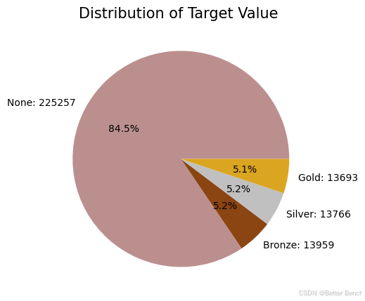
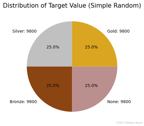
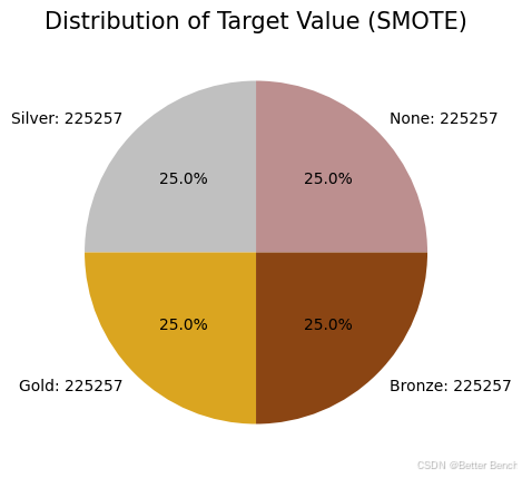
在下面的单元格中，我们使用三种不同的算法（k近邻、高斯朴素贝叶斯和决策树）和两种不同的重采样技术（随机重采样和SMOTE重采样）训练了六个不同的模型。然后，我们比较了六种不同模型的精度。我们使用重采样是因为我们的目标变量是不平衡的。随机重采样是欠采样方法，使所有目标值有9800个样本；SMOTE重采样是少数类的过采样方法，使所有目标值有185547个样本。

3.3.6 简单随机抽样

# Sets all target values to have a count of 9,800, since silver has the least samples
random_resampled_df = combined_df.groupby('target').apply(lambda x: x.sample(n=9800)).reset_index(drop = True)

# Create pie chart of distribution
piedist(random_resampled_df, title = '(Simple Random)')

请添加图片描述

3.3.7 SMOTE Sampling

from collections import Counter
from imblearn.over_sampling import SMOTE

# Oversampling minority target values
X = combined_df.drop(["target"], axis =1)
y = combined_df["target"]

sm = SMOTE(sampling_strategy = 'all', random_state=3000)
X_resampled, y_resampled = sm.fit_resample(X, y)

# Create new dataframe of resampled values
df_target_smote = pd.DataFrame(y_resampled, columns =['target'])
smote_resampled_df = pd.concat([X_resampled, df_target_smote], axis=1)

# Create pie plot of target value distribution after smote resampling
piedist(smote_resampled_df, title = '(SMOTE)')

请添加图片描述

3.3.8 抽样方法比较

正如从下面的输出中看到的，对于kNN和决策树，SMOTE重采样数据比使用kNN和决策树分类器的随机重采样数据具有更高的精度。随机重采样数据和非随机重采样数据的kNN准确率从48.06%提高到88.45%。随机重采样数据和SMOTE重采样数据的决策树准确率由57.68%提高到86.38%。然而，高斯朴素贝叶斯在两种重采样技术之间差异不大，总体而言，该模型的准确率远低于kNN和Decision Tree，平均准确率低于30%。

# Define dictionary of sampling methods for easy use later
sampling_techniques = {"Random Sampling" : random_resampled_df, 
                       "SMOTE Sampling" : smote_resampled_df}


def best_sampling(): 
    # Loop through sampling methods
    for sampling_name, df in sampling_techniques.items():
        
        # Redefine feature and target for each resampled dataset
        features = df.drop(["target"], axis=1)
        target = df["target"]
        
        # Split into train and test sets
        X_train, X_test, y_train, y_test = train_test_split(features, target, random_state=3000)
        y_train = np.ravel(y_train)
        y_test = np.ravel(y_test)
    
        # Train and return accuracy score, add to performance metrics dataframe
        for name, estimator in estimators.items():
            model = estimator.fit(X=X_train, y=y_train)
            accuracy = model.score(X_test, y_test)
            print(f'{name}: \n\t Classification accuracy on the test data with {sampling_name}: {accuracy:.2%}\n')
            predicted = model.predict(X=X_test)
            metrics(sampling_name, name, model, predicted, y_test)

best_sampling()

k-Nearest Neighbor: 
	 Classification accuracy on the test data with Random Sampling: 58.71%

Gaussian Naive Bayes: 
	 Classification accuracy on the test data with Random Sampling: 27.47%

Decision Tree: 
	 Classification accuracy on the test data with Random Sampling: 65.14%

k-Nearest Neighbor: 
	 Classification accuracy on the test data with SMOTE Sampling: 90.85%

Gaussian Naive Bayes: 
	 Classification accuracy on the test data with SMOTE Sampling: 27.64%

Decision Tree: 
	 Classification accuracy on the test data with SMOTE Sampling: 90.94%

# SMOTE resampled dataset without log transformations
features = smote_resampled_df.drop(["target"], axis=1)
target = smote_resampled_df["target"]

3.3.9 数据变换

除了对数变换，还想使用标准标量和最小最大标量，看看它们是否能更有效地校正原始数据集中的值分布。对于这一部分，比较了标量器在对数转换数据和原始特征（没有转换）上的性能。

from sklearn.preprocessing import MinMaxScaler
from sklearn.preprocessing import StandardScaler
from sklearn.model_selection import train_test_split

# Define tests to perform
# Scaling before log and normalized transformations
scalers = {"Min Max Scaler" : MinMaxScaler(), "Standard Scaler" : StandardScaler()}
# Scaling after log and normalized transformations
scalers_log = {"Min Max Scaler (Log)": MinMaxScaler(), "Standard Scaler (Log)": StandardScaler()}

def best_preprocessing(scalers_dict, features, target): 
    """ scalers_dict: either scalers or scalers log for scaling methods to test
        features: predefined features dataframe (from SMOTE resampling)
        target: predefined target series (from SMOTE resampling)
    """
    # Split into train and test sets
    X_train, X_test, y_train, y_test = train_test_split(features, target, random_state=3000)
    
    # Loop through and test min max and standard scaler
    for scaling_name, scaling_method in scalers_dict.items():
        
        # Define, fit, and test scaling method
        scaler = scaling_method
        scaler.fit(X_train) 
        X_train_scaled = scaler.transform(X_train) 
        X_test_scaled = scaler.transform(X_test)
        
        # Use trained scaler to test the three models
        for name, estimator in estimators.items():
            model = estimator.fit(X=X_train_scaled, y=y_train)
            accuracy_train = model.score(X_train_scaled, y_train)
            accuracy_test = model.score(X_test_scaled, y_test)
            
            # Add performance metrics to performance dataframe
            predicted = model.predict(X=X_test)
            metrics(scaling_name, name, model, predicted, y_test)
            
            # Return accuracy scores of different scaling methods
            print(f'{name}:')
            print(f'\t Classification accuracy on the training data with {scaling_name}: {accuracy_train:.2%}')
            print(f'\n\t Classification accuracy on the test data with {scaling_name}: {accuracy_test:.2%}\n')
            continue

3.3.10 测试没有对数转换的标量

在下一个单元格中，使用三种不同的算法（k-Nearest Neighbors，高斯朴素贝叶斯和决策树）和两种不同的缩放技术（Min Max Scaler和Standard Scaler）训练了六个不同的模型，并且已经使用SMOTE对数据进行了重新采样，因为SMOTE比随机重新采样具有更高的精度。最小最大标度器对kNN的准确度略高于标准标度器（84.83% ~ 83.44%）。使用最小最大标量和标准标量，朴素贝叶斯的准确率相同，为32.05%。Min Max Scaler和Standard Scaler的决策树准确率基本相同，但Min Max Scaler略高（86.45% ~ 86.38%）。kNN和朴素贝叶斯（对于最小最大标量和标准标量）没有显示过拟合的迹象；然而，对于两种缩放方法，决策树表明模型可能是过拟合的。这是因为决策树分类器的训练数据的准确率为99.9%，而测试数据的准确率仅为86%左右；这表明，对于所拥有的信息量来说，构建的决策树模型过于复杂，并且过于接近的训练集的特殊性。

best_preprocessing(scalers, features, target)

k-Nearest Neighbor:
	 Classification accuracy on the training data with Min Max Scaler: 91.87%

	 Classification accuracy on the test data with Min Max Scaler: 87.88%

Gaussian Naive Bayes:
	 Classification accuracy on the training data with Min Max Scaler: 32.44%

	 Classification accuracy on the test data with Min Max Scaler: 32.24%

Decision Tree:
	 Classification accuracy on the training data with Min Max Scaler: 99.97%

	 Classification accuracy on the test data with Min Max Scaler: 90.90%

k-Nearest Neighbor:
	 Classification accuracy on the training data with Standard Scaler: 91.19%

	 Classification accuracy on the test data with Standard Scaler: 87.00%

Gaussian Naive Bayes:
	 Classification accuracy on the training data with Standard Scaler: 32.44%

	 Classification accuracy on the test data with Standard Scaler: 32.24%

Decision Tree:
	 Classification accuracy on the training data with Standard Scaler: 99.97%

	 Classification accuracy on the test data with Standard Scaler: 90.89%

3.3.11 用对数变换测试标量

这里使用的数据已经使用对数转换进行了转换，以防止偏度。偏性存在于的连续数值变量中，因此在使用对数变换时，使这些特征更符合正态分布。在下一个单元格中，使用三种不同的算法（k-Nearest Neighbors，高斯朴素贝叶斯和决策树）和两种不同的缩放技术（Min Max Scaler和Standard Scaler）训练了六个不同的模型，并且已经使用SMOTE对数据进行了重新采样，因为SMOTE比随机重新采样具有更高的精度。最小最大标度器对kNN的准确度略高于标准标度器（85.61% ~ 84.44%）。使用最小最大标量和标准标量，朴素贝叶斯的准确率相同，为84.96%。Min Max Scaler和Standard Scaler的决策树准确率基本相同，但Min Max Scaler略高（86.39% ~ 86.34%）。最小最大标量和标准标量的kNN和朴素贝叶斯都没有显示出过拟合的迹象，然而，使用两种缩放方法的决策树表明模型可能是过拟合的。这是因为Decision Tree分类器的训练数据的准确率为99.9%，而测试数据的准确率仅为86%左右。

# Define features and target dataframes from previous, log-transformed dataset
features = df_log_transf.drop(["target"], axis=1)
target = df_log_transf["target"]

# Find best preprocessing (scaler vs minmax of log-transformed data)
best_preprocessing(scalers_log, features, target)

k-Nearest Neighbor:
	 Classification accuracy on the training data with Min Max Scaler (Log): 91.79%

	 Classification accuracy on the test data with Min Max Scaler (Log): 88.88%

Gaussian Naive Bayes:
	 Classification accuracy on the training data with Min Max Scaler (Log): 84.37%

	 Classification accuracy on the test data with Min Max Scaler (Log): 84.60%

Decision Tree:
	 Classification accuracy on the training data with Min Max Scaler (Log): 100.00%

	 Classification accuracy on the test data with Min Max Scaler (Log): 88.72%

k-Nearest Neighbor:
	 Classification accuracy on the training data with Standard Scaler (Log): 90.90%

	 Classification accuracy on the test data with Standard Scaler (Log): 87.93%

Gaussian Naive Bayes:
	 Classification accuracy on the training data with Standard Scaler (Log): 84.37%

	 Classification accuracy on the test data with Standard Scaler (Log): 84.60%

Decision Tree:
	 Classification accuracy on the training data with Standard Scaler (Log): 100.00%

	 Classification accuracy on the test data with Standard Scaler (Log): 88.72%

3.3.12 特征选择：递归特征消除

# Define features and target for feature selection and hyperparameter tuning
features = smote_resampled_df.drop(["target"], axis=1)
target = smote_resampled_df["target"]

from sklearn.feature_selection import RFE
from sklearn.tree import DecisionTreeRegressor 

def RFE_feature_selection(estimator, n):
    """ estimator: define which modeling technique (kNN, tree, naive bayes),
        n: define number of features to select """
    method = estimators[estimator]
    X_train, X_test, y_train, y_test = train_test_split(features, target, random_state = 3000)
    
    # Get the most important features using RFE
    important_features = RFE(DecisionTreeClassifier(random_state = 3000), n_features_to_select = n)
    
    # Fit the RFE selector to the training data 
    important_features.fit(X_train, y_train)
    
    # Transform training and testing sets so that only the important selected features remain 
    X_train_selected = important_features.transform(X_train)
    X_test_selected = important_features.transform(X_test)
    
    # Apply method to the training data 
    model = method.fit(X=X_train_selected, y=y_train)
    
    print("Selected features after RFE: ")
    
    # Iterates through the number of columns in the df 
    for i in range(len(features.columns)): 
        
        # If the value corresponding with the column of the feature is true, the feature was used in the model
        if (important_features.support_[i] == True): 
            print("\t", features.columns[i])
            
    # Prints accuracy for the model on the training and testing sets 
    print("\n" + "Performance with selected features: ")
    print("\t" + "Accuracy for the training set: ", model.score(X_train_selected, y_train))
    print("\t" + "Accuracy for the testing set: ", model.score(X_test_selected, y_test))
    
    # Evaluate performance metrics and add to performance dataframe
    predicted = model.predict(X=X_test_selected)
    metrics('Feature Selection', estimator, model, predicted, y_test)

用kNN分类器进行特征选择

n-values we tried: 4, 5, 6 7, 8, 9, 10

利用递归特征消去（RFE）确定了三种不同分类模型的最重要特征。对于kNN分类器，在国家、年份、事件、GDP、年龄、BMI、身高和体重这8个特征上获得了最高的准确率。在测试集上的准确率约为88.29%，模型不存在过拟合现象。这表明的模型中最重要的8个特征是上面列出的特征，这比没有特征选择的kNN模型产生更高的精度。

RFE_feature_selection('k-Nearest Neighbor', 8)

Selected features after RFE: 
	 Country
	 Year
	 Event
	 GDP
	 Age
	 BMI
	 Height
	 Weight

Performance with selected features: 
	Accuracy for the training set:  0.9345636317628309
	Accuracy for the testing set:  0.9068930155333685

基于决策树分类器的特征选择

n-values we tried: 4, 5, 6, 7, 8, 9, 10

对于决策树分类器，获得了9个特征的最高准确率，这9个特征包括国家、年份、运动、事件、GDP、年龄、BMI、身高和体重。在测试集上的准确率约为86.09%，而在训练集上的准确率接近100%，表明模型是过拟合的。RFE特征选择表明，最重要的9个特征是上面列出的特征，但与没有特征选择的数据相比，模型的准确率没有明显提高。

RFE_feature_selection('Decision Tree', 9)

Selected features after RFE: 
	 Country
	 Year
	 Sport
	 Event
	 GDP
	 Age
	 BMI
	 Height
	 Weight

Performance with selected features: 
	Accuracy for the training set:  0.9994951863049973
	Accuracy for the testing set:  0.8609840094423515


C:\Users\feiyu\anaconda3\lib\site-packages\pandas\core\indexing.py:1637: SettingWithCopyWarning: 
A value is trying to be set on a copy of a slice from a DataFrame

See the caveats in the documentation: https://pandas.pydata.org/pandas-docs/stable/user_guide/indexing.html#returning-a-view-versus-a-copy
  self._setitem_single_block(indexer, value, name)

朴素贝叶斯分类器的特征选择

n-values tried: 3, 4, 5, 6, 7, 8, 9

对于朴素贝叶斯分类器，在Year， Event, Age， BMI和Height这5个特征上获得了最高的准确率。在测试集上的准确率约为30.66%，模型不存在过拟合现象。这表明使用朴素贝叶斯的模型中最重要的5个特征是上面列出的特征，这比没有特征选择的模型产生略高的精度（不到1%）。

RFE_feature_selection('Gaussian Naive Bayes', 5)

Selected features after RFE: 
	 Year
	 Event
	 Age
	 BMI
	 Height

Performance with selected features: 
	Accuracy for the training set:  0.3053997100465111
	Accuracy for the testing set:  0.3065638355780476


C:\Users\feiyu\anaconda3\lib\site-packages\pandas\core\indexing.py:1637: SettingWithCopyWarning: 
A value is trying to be set on a copy of a slice from a DataFrame

See the caveats in the documentation: https://pandas.pydata.org/pandas-docs/stable/user_guide/indexing.html#returning-a-view-versus-a-copy
  self._setitem_single_block(indexer, value, name)

3.4. 模型优化

。。。。

3.4.1 使用GridSearch进行超参数调优

from sklearn.model_selection import GridSearchCV

def grid_search(estimator, param_grid):
    """ estimator: model to test with (knn, tree, naive bayes)
        param_grid: dictionary of different parameters and values to testa nd compare"""
    # Use grid search to find best parameters
    method = estimators[estimator]
    grid_search = GridSearchCV(method, param_grid, cv=5)
    
    # Split into train and test sets, fit with grid search
    X_train, X_test, y_train, y_test = train_test_split(features, target, random_state = 3000)
    grid_search.fit(X=X_train, y=y_train)
    
    # Print resulting best parameters and evaluation metrics
    print("Best parameters: ", grid_search.best_params_)
    
    #print("Best cross-validation score: ", grid_search.best_score_)
    print("Test set score: ", grid_search.score(X_test, y_test))
    
    # Evaluate performance metrics and add to performance dataframe
    predicted = grid_search.predict(X=X_test)
    metrics('Grid Search CV', estimator, grid_search, predicted, y_test)

kNN分类器的GridSearch

对于kNN，测试了参数n_neighbors、weights和metric，以便找到产生最准确的kNN测试集分数的参数的正确组合。准确度最高的是度量为曼哈顿，1个邻居，权重为均匀，准确度为93.45%。

# Hyperparameters to test
param_grid = {"n_neighbors":[1, 5, 15, 25, 55], "weights":["uniform", "distance"], "metric":["euclidean", "manhattan", "minkowski"]}

grid_search('k-Nearest Neighbor', param_grid)

Best parameters:  {'metric': 'manhattan', 'n_neighbors': 1, 'weights': 'uniform'}
Test set score:  0.9344802125606989


C:\Users\feiyu\anaconda3\lib\site-packages\pandas\core\indexing.py:1637: SettingWithCopyWarning: 
A value is trying to be set on a copy of a slice from a DataFrame

See the caveats in the documentation: https://pandas.pydata.org/pandas-docs/stable/user_guide/indexing.html#returning-a-view-versus-a-copy
  self._setitem_single_block(indexer, value, name)

决策树分类器的GridSearch

对于决策树模型，测试了参数标准max_depth和min_samples_leaf，以便确定产生最高测试集精度的最佳参数。结果是作为熵的标准，max_depth为55，min_samples_leaf为1，这给的测试集的准确率得分为86.75%。

# Hyperparameters to test
param_grid = {"criterion":["gini", "entropy"], "max_depth":[5, 11, 15, 25, 35, 55], "min_samples_leaf":[1, 2, 3, 4, 5, 6, 7, 8, 9, 10]}

grid_search('Decision Tree', param_grid)

Best parameters:  {'criterion': 'entropy', 'max_depth': 55, 'min_samples_leaf': 1}
Test set score:  0.8674675419166034


C:\Users\feiyu\anaconda3\lib\site-packages\pandas\core\indexing.py:1637: SettingWithCopyWarning: 
A value is trying to be set on a copy of a slice from a DataFrame

See the caveats in the documentation: https://pandas.pydata.org/pandas-docs/stable/user_guide/indexing.html#returning-a-view-versus-a-copy
  self._setitem_single_block(indexer, value, name)

朴素贝叶斯分类器的GridSearch

对于朴素贝叶斯分类器，测试了参数var_smoothing，看看哪个值产生最准确的模型。当var_smoothing = 0.019时，测试集得分为29.60%。

# Hyperparameters to test
param_grid = {'var_smoothing': np.logspace(0,-9, num=100)}

grid_search('Gaussian Naive Bayes', param_grid)

Best parameters:  {'var_smoothing': 0.01873817422860384}
Test set score:  0.29601664268352496


C:\Users\feiyu\anaconda3\lib\site-packages\sklearn\metrics\_classification.py:1245: UndefinedMetricWarning: Precision and F-score are ill-defined and being set to 0.0 in labels with no predicted samples. Use `zero_division` parameter to control this behavior.
  _warn_prf(average, modifier, msg_start, len(result))
C:\Users\feiyu\anaconda3\lib\site-packages\sklearn\metrics\_classification.py:1245: UndefinedMetricWarning: Precision and F-score are ill-defined and being set to 0.0 in labels with no predicted samples. Use `zero_division` parameter to control this behavior.
  _warn_prf(average, modifier, msg_start, len(result))
C:\Users\feiyu\anaconda3\lib\site-packages\sklearn\metrics\_classification.py:1245: UndefinedMetricWarning: Precision and F-score are ill-defined and being set to 0.0 in labels with no predicted samples. Use `zero_division` parameter to control this behavior.
  _warn_prf(average, modifier, msg_start, len(result))
C:\Users\feiyu\anaconda3\lib\site-packages\pandas\core\indexing.py:1637: SettingWithCopyWarning: 
A value is trying to be set on a copy of a slice from a DataFrame

See the caveats in the documentation: https://pandas.pydata.org/pandas-docs/stable/user_guide/indexing.html#returning-a-view-versus-a-copy
  self._setitem_single_block(indexer, value, name)

3.5. 模型测试

3.5.1 对比出最佳模型

performance

		Base			Random Sampling			SMOTE Sampling			Min Max Scaler	...	Min Max Scaler (Log)	Standard Scaler (Log)			Feature Selection			Grid Search CV
		k-Nearest Neighbor	Gaussian Naive Bayes	Decision Tree	k-Nearest Neighbor	Gaussian Naive Bayes	Decision Tree	k-Nearest Neighbor	Gaussian Naive Bayes	Decision Tree	k-Nearest Neighbor	...	Decision Tree	k-Nearest Neighbor	Gaussian Naive Bayes	Decision Tree	k-Nearest Neighbor	Gaussian Naive Bayes	Decision Tree	k-Nearest Neighbor	Gaussian Naive Bayes	Decision Tree
0	precision	0.452998	0.053008	0.549060	0.473999	0.392956	0.620392	0.878263	0.386609	0.866055	0.262693	...	0.076520	0.071429	0.038249	0.063149	0.876671	0.298182	0.862215	0.936133	0.384475	0.864842
	recall	0.396735	0.031583	0.569908	0.604745	0.228790	0.636108	0.951606	0.230265	0.876547	0.002565	...	0.155429	0.000355	0.085877	0.479063	0.950032	0.298793	0.873162	0.965898	0.231257	0.880017
	f1-score	0.423004	0.039582	0.559290	0.531449	0.289199	0.628152	0.913465	0.288625	0.871269	0.005081	...	0.102552	0.000706	0.052925	0.111589	0.911879	0.298487	0.867654	0.950782	0.288802	0.872364
	support	2818.000000	2818.000000	2818.000000	2487.000000	2487.000000	2487.000000	46390.000000	46390.000000	46390.000000	46390.000000	...	2818.000000	2818.000000	2818.000000	2818.000000	46390.000000	46390.000000	46390.000000	46390.000000	46390.000000	46390.000000
1	precision	0.336095	0.000000	0.456111	0.443400	0.000000	0.547983	0.863609	0.000000	0.849057	0.278146	...	0.061800	0.000000	0.000000	0.060004	0.862027	0.284736	0.841556	0.926427	0.000000	0.852848
	recall	0.218546	0.000000	0.519815	0.474638	0.000000	0.563205	0.938120	0.000000	0.857683	0.000902	...	0.061562	0.000000	0.000000	0.248557	0.936402	0.164268	0.850359	0.957150	0.000000	0.859058
	f1-score	0.264864	0.000000	0.485884	0.458487	0.000000	0.555489	0.899324	0.000000	0.853348	0.001798	...	0.061681	0.000000	0.000000	0.096670	0.897676	0.208341	0.845934	0.941538	0.000000	0.855941
	support	2599.000000	2599.000000	2599.000000	2484.000000	2484.000000	2484.000000	46558.000000	46558.000000	46558.000000	46558.000000	...	2599.000000	2599.000000	2599.000000	2599.000000	46558.000000	46558.000000	46558.000000	46558.000000	46558.000000	46558.000000
2	precision	0.354732	0.000000	0.436707	0.453237	0.000000	0.553055	0.863320	0.000000	0.846485	0.186296	...	0.049048	0.000000	0.000000	0.068684	0.862498	0.283025	0.842261	0.923837	0.268287	0.849883
	recall	0.201352	0.000000	0.478212	0.417910	0.000000	0.570481	0.936359	0.000000	0.860257	0.001872	...	0.159654	0.000000	0.000000	0.031555	0.934465	0.290225	0.853499	0.957817	0.161824	0.860602
	f1-score	0.256890	0.000000	0.456518	0.434858	0.000000	0.561633	0.898357	0.000000	0.853315	0.003708	...	0.075042	0.000000	0.000000	0.043243	0.897040	0.286580	0.847843	0.940520	0.201879	0.855209
	support	2662.000000	2662.000000	2662.000000	2412.000000	2412.000000	2412.000000	46464.000000	46464.000000	46464.000000	46464.000000	...	2662.000000	2662.000000	2662.000000	2662.000000	46464.000000	46464.000000	46464.000000	46464.000000	46464.000000	46464.000000
3	precision	0.906148	0.851892	0.938963	0.653670	0.265685	0.598008	0.956197	0.266361	0.903347	0.248981	...	0.861406	0.851774	0.845118	0.898936	0.952414	0.339054	0.900088	0.954307	0.282970	0.904338
	recall	0.953180	0.969311	0.924343	0.471659	0.918080	0.546545	0.711174	0.911737	0.868278	0.995578	...	0.696315	0.999720	0.877006	0.409364	0.709310	0.474434	0.866999	0.856508	0.795015	0.870250
	f1-score	0.929069	0.906816	0.931595	0.547945	0.412109	0.571120	0.815682	0.412277	0.885465	0.398342	...	0.770112	0.919836	0.860766	0.562550	0.813079	0.395479	0.883234	0.902767	0.417381	0.886967
	support	46433.000000	46433.000000	46433.000000	2417.000000	2417.000000	2417.000000	46135.000000	46135.000000	46135.000000	46135.000000	...	46433.000000	46433.000000	46433.000000	46433.000000	46135.000000	46135.000000	46135.000000	46135.000000	46135.000000	46135.000000
all	accuracy	0.852675	0.827286	0.864947	0.492959	0.284490	0.579388	0.884622	0.284268	0.865678	0.248880	...	0.611884	0.851574	0.751468	0.386851	0.882860	0.306564	0.860984	0.934480	0.296017	0.867468
macro avg	precision	0.512493	0.226225	0.595210	0.506077	0.164660	0.579859	0.890347	0.163243	0.866236	0.244029	...	0.262193	0.230801	0.220842	0.272693	0.888402	0.301249	0.861530	0.935176	0.233933	0.867978
	recall	0.442453	0.250223	0.623069	0.492238	0.286717	0.579085	0.884315	0.285501	0.865691	0.250229	...	0.268240	0.250019	0.240721	0.292135	0.882552	0.306930	0.861005	0.934343	0.297024	0.867482
	f1-score	0.468457	0.236599	0.608322	0.493185	0.175327	0.579098	0.881707	0.175225	0.865849	0.102232	...	0.252347	0.230136	0.228423	0.203513	0.879919	0.297222	0.861166	0.933902	0.227016	0.867620
	support	54512.000000	54512.000000	54512.000000	9800.000000	9800.000000	9800.000000	185547.000000	185547.000000	185547.000000	185547.000000	...	54512.000000	54512.000000	54512.000000	54512.000000	185547.000000	185547.000000	185547.000000	185547.000000	185547.000000	185547.000000
weighted avg	precision	0.828616	0.728377	0.871259	0.505446	0.165249	0.579945	0.890222	0.162888	0.866161	0.244030	...	0.743038	0.729229	0.721844	0.775188	0.888280	0.301175	0.861451	0.935137	0.233667	0.867907
	recall	0.852675	0.827286	0.864947	0.492959	0.284490	0.579388	0.884622	0.284268	0.865678	0.248880	...	0.611884	0.851574	0.751468	0.386851	0.882860	0.306564	0.860984	0.934480	0.296017	0.867468
	f1-score	0.838416	0.774467	0.867899	0.493251	0.175031	0.579296	0.881820	0.174671	0.865806	0.101695	...	0.667884	0.783548	0.735932	0.491666	0.880033	0.297002	0.861117	0.933954	0.226539	0.867578
	support	54512.000000	54512.000000	54512.000000	9800.000000	9800.000000	9800.000000	185547.000000	185547.000000	185547.000000	185547.000000	...	54512.000000	54512.000000	54512.000000	54512.000000	185547.000000	185547.000000	185547.000000	185547.000000	185547.000000	185547.000000

25 rows × 27 columns

# Save evaluation metrics dataframe as csv
performance.to_csv('model_evaluation.csv')

最佳表现模型：

为了找到性能最好的模型，在性能数据框架中对每个模型的性能取平均值。发现三个最高的平均值属于网格搜索kNN（平均分：93.45%），SMOTE采样kNN（88.54%）和超参数调谐kNN（88.36%）。一般来说，kNN估计器的性能最好。

# Define subset of original dataframe without support metric value
no_support = []
for row in performance.index:
    if row[1] != 'support':
        no_support.append(row)
final_vals = performance.loc[no_support]

# Find mean of each model using the metric scores and sort in descending order
means = final_vals.mean(axis=0)
means.sort_values(ascending=False)

Grid Search CV         k-Nearest Neighbor      0.934482
SMOTE Sampling         k-Nearest Neighbor      0.885428
Feature Selection      k-Nearest Neighbor      0.883600
Grid Search CV         Decision Tree           0.867675
SMOTE Sampling         Decision Tree           0.865906
Feature Selection      Decision Tree           0.861213
Base                   Decision Tree           0.663266
Random Sampling        Decision Tree           0.579380
Base                   k-Nearest Neighbor      0.552074
Random Sampling        k-Nearest Neighbor      0.496953
Standard Scaler (Log)  k-Nearest Neighbor      0.356353
Base                   Gaussian Naive Bayes    0.353824
Min Max Scaler (Log)   k-Nearest Neighbor      0.351436
                       Decision Tree           0.344663
Standard Scaler (Log)  Gaussian Naive Bayes    0.337402
Min Max Scaler (Log)   Gaussian Naive Bayes    0.335719
Standard Scaler (Log)  Decision Tree           0.309593
Feature Selection      Gaussian Naive Bayes    0.302016
Grid Search CV         Gaussian Naive Bayes    0.254847
Min Max Scaler         Decision Tree           0.218359
Random Sampling        Gaussian Naive Bayes    0.212778
SMOTE Sampling         Gaussian Naive Bayes    0.211891
Min Max Scaler         k-Nearest Neighbor      0.201365
Standard Scaler        Decision Tree           0.182212
Min Max Scaler         Gaussian Naive Bayes    0.143427
Standard Scaler        Gaussian Naive Bayes    0.143427
                       k-Nearest Neighbor      0.142986
dtype: float64