


ArcLoss实现
以MNIST数据集为例
前言
尝试了很多版本,目前没有找到一个适合CIFAR10数据集的网络模型0.0
V0
网络结构
self.hidden_layer = nn.Sequential(
    ConvLayer(1, 16, 3, 1, 0),
    nn.MaxPool2d(2),
    ConvLayer(16, 32, 3, 1, 0),
    ConvLayer(32, 64, 3, 1, 0),
    ConvLayer(64, 128, 3, 1, 0),
    ConvLayer(128, 256, 3, 1, 0),
)

self.fc = nn.Sequential(
    nn.Linear(256 * 5 * 5, 2)
)
参数
data_loader = DataLoader(dataset=mnist_data, shuffle=True, batch_size=256)
opt_net = torch.optim.Adam(net.parameters())
opt_arc = torch.optim.Adam(arc.parameters())
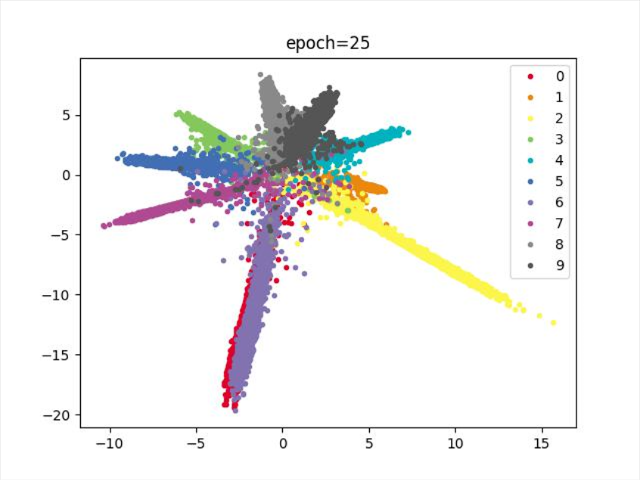
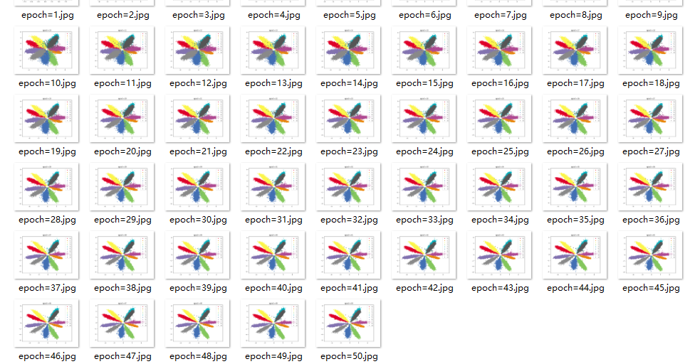
效果
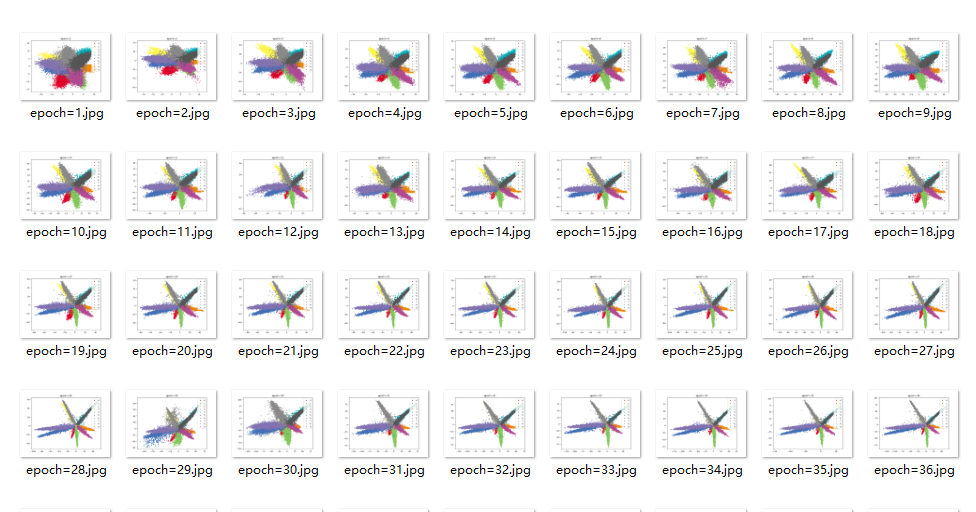
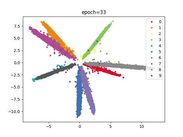
训练到中途,数据不稳定
训练100次,无法进一步划分类别
结论
类别无法完全分开,训练到中途,数据图形爆炸
V1
增加网络深度
网络结构
self.hidden_layer = nn.Sequential(
    ConvLayer(1, 32, 5, 1, 2),
    ConvLayer(32, 64, 5, 1, 2),
    nn.MaxPool2d(2, 2),
    ConvLayer(64, 128, 5, 1, 2),
    ConvLayer(128, 256, 5, 1, 2),
    nn.MaxPool2d(2, 2),
    ConvLayer(256, 512, 5, 1, 2),
    ConvLayer(512, 512, 5, 1, 2),
    nn.MaxPool2d(2, 2),
    ConvLayer(512, 256, 5, 1, 2),
    ConvLayer(256, 128, 5, 1, 2),
    ConvLayer(128, 64, 5, 1, 2),
    nn.MaxPool2d(2, 2)
)

self.fc = nn.Sequential(
    nn.Linear(64, 2)
)
参数
data_loader = DataLoader(dataset=mnist_data, shuffle=True, batch_size=256)
opt_net = torch.optim.Adam(net.parameters())
opt_arc = torch.optim.Adam(arc.parameters())
效果
结论
持续十多轮,无法进一步减少损失,尝试更换优化器,实现降低损失
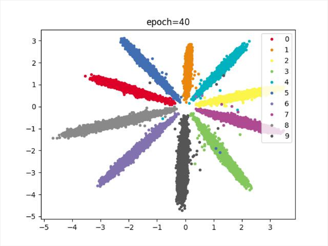
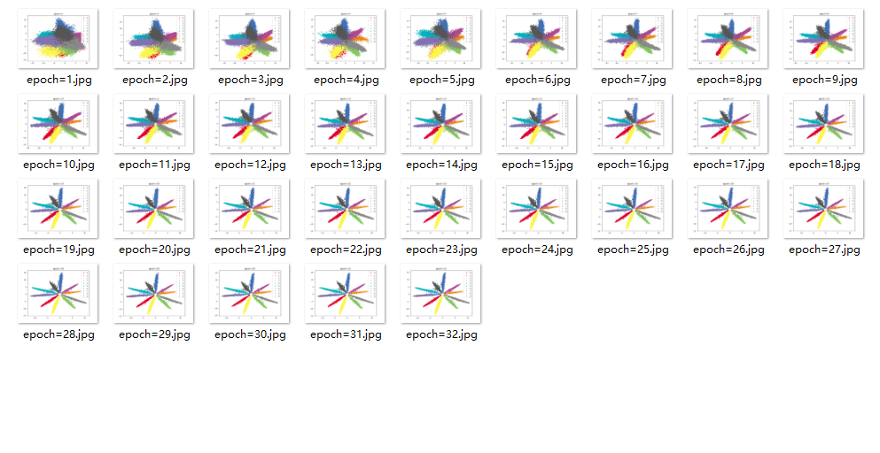
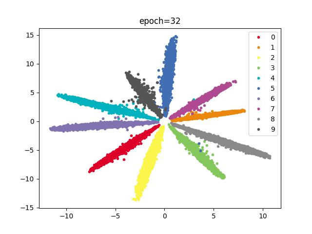
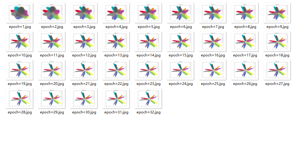
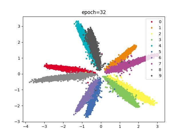
V1.1(最佳)
V1基础上调整优化器Adam–>SGD,其余条件不变
参数
data_loader = DataLoader(dataset=mnist_data, shuffle=True, batch_size=256)
opt_net = torch.optim.SGD(net.parameters(), lr=0.001, momentum=0.9)
scheduler = torch.optim.lr_scheduler.StepLR(opt_net, 20, gamma=0.8)
opt_arc = torch.optim.SGD(arc.parameters(), lr=0.5)
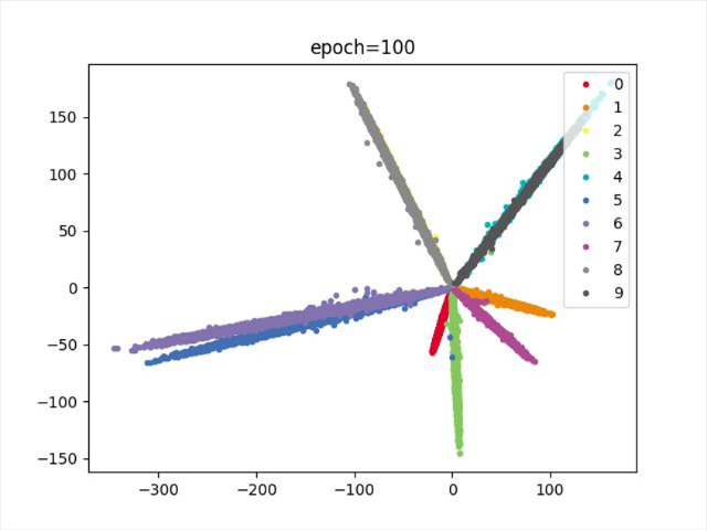
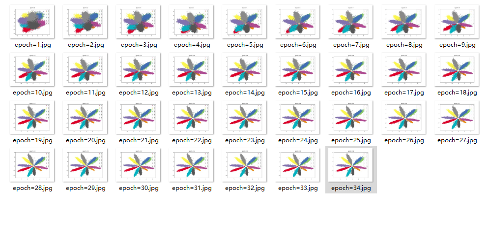
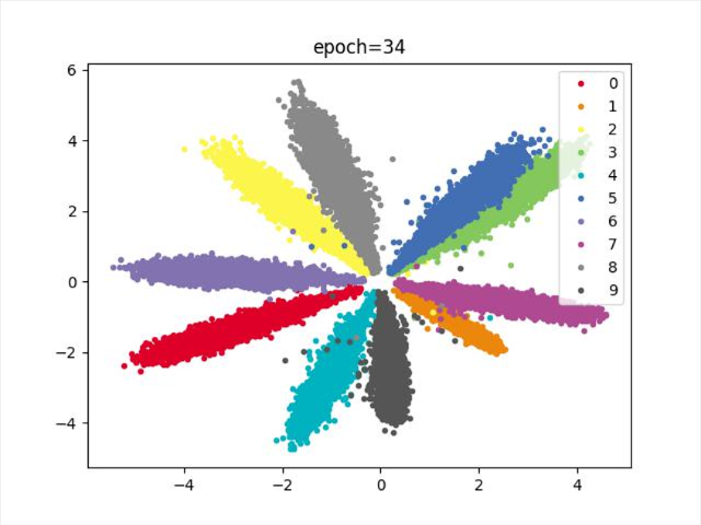
效果
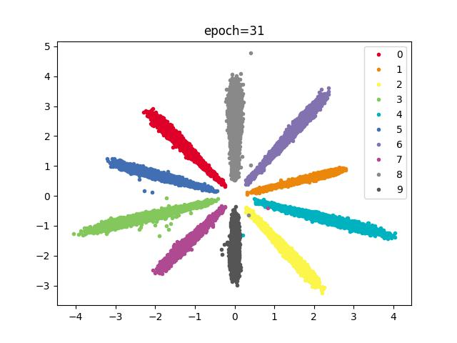
结论
分类效果明显,训练速度减慢,SGD优化器在合适的参数下,比Adam分类效果更好
V1.1.2(佳)
V1.1基础上减少网络宽度,其余条件不变
网络结构
self.hidden_layer = nn.Sequential(
    ConvLayer(1, 32, 5, 1, 2),
    ConvLayer(32, 32, 5, 1, 2),
    nn.MaxPool2d(2, 2),
    ConvLayer(32, 64, 5, 1, 2),
    ConvLayer(64, 64, 5, 1, 2),
    nn.MaxPool2d(2, 2),
    ConvLayer(64, 128, 5, 1, 2),
    ConvLayer(128, 128, 5, 1, 2),
    nn.MaxPool2d(2, 2),
    ConvLayer(128, 256, 5, 1, 2),
    ConvLayer(256, 128, 5, 1, 2),
    ConvLayer(128, 64, 5, 1, 2),
    nn.MaxPool2d(2, 2)
)

self.fc = nn.Sequential(
    nn.Linear(64, 2)
)
效果
结论
分类明显,宽度减少,收敛速度较慢
V1.1.3
V1.1.2基础上,网络全连接改为卷积,其余条件不变
网络结构
self.hidden_layer = nn.Sequential(
    ConvLayer(1, 32, 5, 1, 2),
    ConvLayer(32, 32, 5, 1, 2),
    nn.MaxPool2d(2, 2),
    ConvLayer(32, 64, 5, 1, 2),
    ConvLayer(64, 64, 5, 1, 2),
    nn.MaxPool2d(2, 2),
    ConvLayer(64, 128, 5, 1, 2),
    ConvLayer(128, 128, 5, 1, 2),
    nn.MaxPool2d(2, 2),
    ConvLayer(128, 256, 5, 1, 2),
    ConvLayer(256, 128, 5, 1, 2),
    ConvLayer(128, 64, 5, 1, 2),
    nn.MaxPool2d(2, 2)
)

self.fc = nn.Sequential(
    # nn.Linear(64, 2)
    nn.Conv2d(64, 2, 5, 1, 2)
)
效果
结论
存在重合类别,效果没有全连接好
V1.1.4
V1.1基础上,修改学习率
参数
data_loader = DataLoader(dataset=mnist_data, shuffle=True, batch_size=256)
opt_net = torch.optim.SGD(net.parameters(), lr=0.01, momentum=0.9)
scheduler = torch.optim.lr_scheduler.StepLR(opt_net, 20, gamma=0.8)
opt_arc = torch.optim.SGD(arc.parameters(), lr=0.5)
效果
结论
类别存在重合
V1.2
V1.1基础上减少网络层数,其余条件不变
网络结构
self.hidden_layer = nn.Sequential(
    ConvLayer(1, 32, 3, 1, 1),
    ConvLayer(32, 64, 3, 1, 2),
    nn.MaxPool2d(2, 2),
    ConvLayer(64, 128, 3, 1, 1),
    ConvLayer(128, 256, 3, 1, 2),
    nn.MaxPool2d(2, 2),
    ConvLayer(256, 256, 3, 1, 1),
    ConvLayer(256, 128, 3, 1, 2),
    nn.MaxPool2d(2, 2)
)

self.fc = nn.Sequential(
    nn.Linear(128 * 5 * 5, 2)
)
效果
结论
训练速度较快,分类收敛速度不如较深层的网络结构,类别存在重合
V1.2.2
相比V1.2条件,更换网络宽度,减少参数
网络结构
self.hidden_layer = nn.Sequential(
    ConvLayer(1, 32, 5, 1, 2),
    ConvLayer(32, 32, 5, 1, 2),
    nn.MaxPool2d(2, 2),
    ConvLayer(32, 64, 5, 1, 2),
    ConvLayer(64, 64, 5, 1, 2),
    nn.MaxPool2d(2, 2),
    ConvLayer(64, 128, 5, 1, 2),
    ConvLayer(128, 128, 5, 1, 2),
    nn.MaxPool2d(2, 2)
)

self.fc = nn.Sequential(
    nn.Linear(128 * 3 * 3, 2)
)
效果
结论
类别存在重合
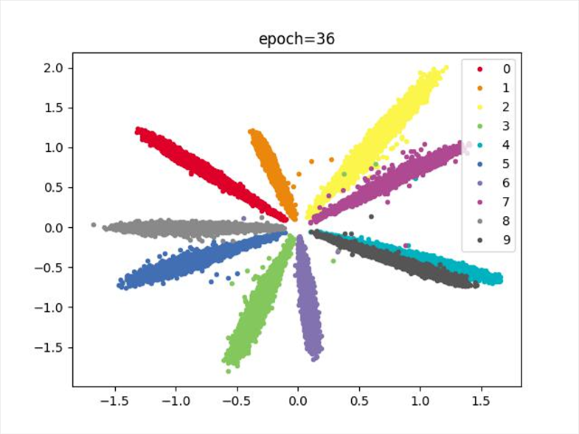
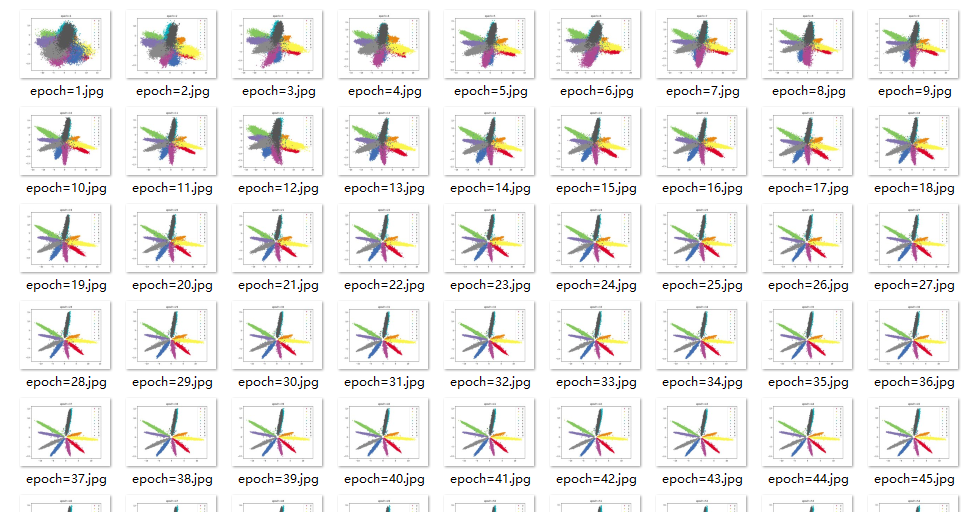
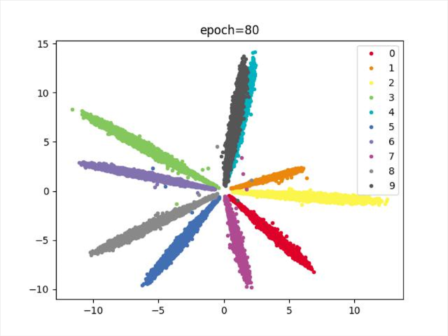
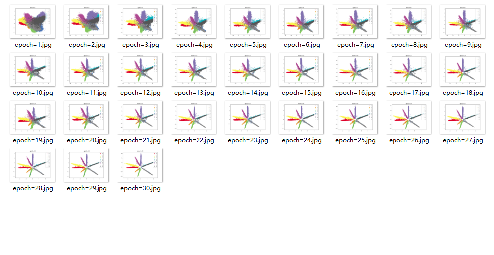
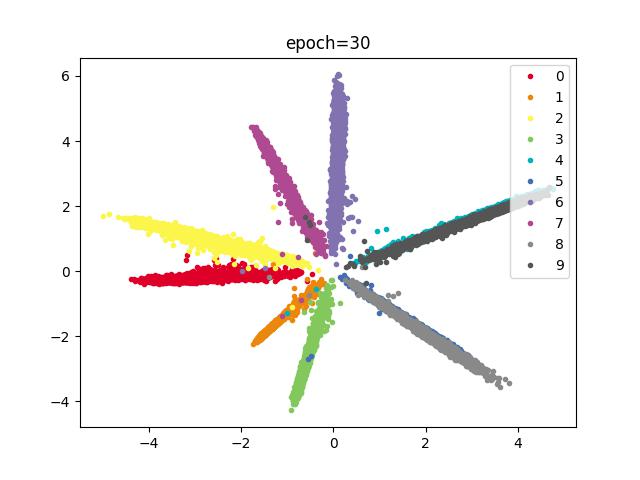
V1.2.3(佳)
V1.2.2基础上,修改网络学习率
参数
data_loader = DataLoader(dataset=mnist_data, shuffle=True, batch_size=256)
opt_net = torch.optim.SGD(net.parameters(), lr=0.01, momentum=0.9)
scheduler = torch.optim.lr_scheduler.StepLR(opt_net, 20, gamma=0.8)
opt_arc = torch.optim.SGD(arc.parameters(), lr=0.5)
效果
结论
分类明显,收敛较快
V1.2.4
V1.2.3基础上,修改批次
参数
data_loader = DataLoader(dataset=mnist_data, shuffle=True, batch_size=512)
opt_net = torch.optim.SGD(net.parameters(), lr=0.01, momentum=0.9)
scheduler = torch.optim.lr_scheduler.StepLR(opt_net, 20, gamma=0.8)
opt_arc = torch.optim.SGD(arc.parameters(), lr=0.5)
效果
结论
批次256–>512,类别存在重合
V2
相比V1条件,更换网络,加深深度,减少宽度,其余条件不变
网络结构
self.hidden_layer = nn.Sequential(
    ConvLayer(1, 32, 5, 1, 2),
    ConvLayer(32, 32, 5, 1, 2),
    nn.MaxPool2d(2, 2),
    ConvLayer(32, 32, 5, 1, 2),
    ConvLayer(32, 32, 5, 1, 2),
    nn.MaxPool2d(2, 2),
    ConvLayer(32, 32, 5, 1, 2),
    ConvLayer(32, 32, 5, 1, 2),
    ConvLayer(32, 32, 5, 1, 2),
    nn.MaxPool2d(2, 2),
    ConvLayer(32, 32, 5, 1, 2),
    ConvLayer(32, 32, 5, 1, 2),
    ConvLayer(32, 32, 5, 1, 2),
    nn.MaxPool2d(2, 2)
)

self.fc = nn.Sequential(
    nn.Linear(32, 2)
)
效果
结论
分类存在重合
V2.1
V2基础上,修改学习率
参数
data_loader = DataLoader(dataset=mnist_data, shuffle=True, batch_size=256)
opt_net = torch.optim.SGD(net.parameters(), lr=0.01, momentum=0.9)
scheduler = torch.optim.lr_scheduler.StepLR(opt_net, 20, gamma=0.8)
opt_arc = torch.optim.SGD(arc.parameters(), lr=0.5)
效果
结论
类别存在重合


 87
87


 被折叠的 条评论
为什么被折叠?
被折叠的 条评论
为什么被折叠?
 到【灌水乐园】发言


