visual modflow flex 9.0

Introduction

Visual MODFLOW (VMOD) Flex is a powerful software package that provides the tools for building three-dimensional groundwater conceptual and numerical models using raw GIS data objects. The conceptual model approach to groundwater modeling allows you to:

·Build a conceptual model of the groundwater system, prior to the simulation - Geologic formation structures, hydrogeologic properties, and  boundary conditions are all designed outside the model grid or mesh; this allows the flexibility to adjust your interpretation of the groundwater system before applying a discretization method and converting to a numerical model.

·Build the model with minimal data pre-processing required - Working with grid-independent data allows you to maximize the use of your existing GIS data and incorporate physical geology and geographic conditions before designing a grid or mesh.

·Generate and simulate regional and local-scaled models - With support for MODFLOW-LGR, you can design local grids around areas of interest, directly within the conceptual model environment. Calculated heads from a regional model can also be used as boundary conditions for local-scaled models.

·Design the correct model faster - The grid-independent raw data is left intact and is not constricted by grid cells or mesh elements when modifying the data and project objective. This allows you to generate multiple numerical models from the same conceptual model.

·Make changes to the model data and immediately see results - The conceptual model environment provides simultaneous 2D and 3D views which are updated whenever changes to the data are made.

This document provides detailed descriptions of all features and functionality available in Visual MODFLOW Flex.

How to get started

ØStudy this Introduction chapter and Program Overview sections to familiarize yourself with the program. ØThen work through the Quick Start Tutorials to familiarize yourself with using VMOD Flex.  These sections cover importing MODFLOW and VMOD Classic projects as well as building new models using the Conceptual Modeling approach. Learning more ØSee Conceptual Modeling Workflow for instructions on building a grid-independent conceptual model using your raw data ØSee Numerical Modeling Workflow for more instructions on working with numerical inputs, translating to MODFLOW packages, and running and analyzing the results. ØSee Working with Multiple Model Scenarios for a better understanding of the various workflows in VMOD Flex. ØSee the Program Overview section for detailed instructions on using VMOD Flex. ØLooking for help beyond what's in this manual?  We have many additional resources for you: üGetting Started with Visual MODFLOW Flex üAn Introduction to Groundwater Modeling Concepts üLinkedIn User’s Group üVisual MODFLOW Flex Frequently Asked Questions (FAQ) üYour Complete Guide to MODFLOW-USG  üAll Tutorials üVisual MODFLOW Flex ReadMe üWhite Papers & Technical Articles

Program Overview

In order to become the most efficient and effective in the Visual MODFLOW Flex environment, it is recommended that you familiarize yourself with a few simple concepts, terminology, and where you can find and access things.

Data Objects

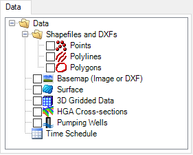
All of the data that you interact with in Visual MODFLOW Flex are referred to as data objects.  These can consist of: ·Raw Data that you have: ·Imported: From polyline or polygon shapefiles, wells from a spreadsheet, surfaces from Surfer .GRD, etc. ·Created: Through digitizing points, polygon, or polylines or by interpolating points to create surfaces ·Conceptual Data Objects: These are generated as you progress through the conceptual modeling workflow, and include: ·Horizons, Structural Zones, Property Zones, and Boundary Conditions. ·Numerical Model Data Objects: These are generated as you progress through a numerical modeling workflow, and include: ·Input: Numerical Grid, Properties (Conductivity, Initial Heads, etc..), Boundary Conditions (a group of river cells, drain cells, pumping  well cells, etc..), Observation Wells, Zone Budget zones, and Particles. ·Output: Calculated Heads, Drawdown, Pathlines, etc. Each data object will have a check box beside it, allowing it to be displayed in different 2D/3D viewers. Data objects can be re-ordered, renamed, or grouped into data folders. To create a data folder, right-click in the Data are Object explorer and select New Folder.  Data folders can be renamed. Each data object also has Settings which can be accessed by right-clicking on the data object in the tree, and selecting Settings. The settings provide access to general properties (statistics, file origin, etc.) and Style settings (symbol colors, shape, labeling, etc.) for those objects displayed in an active viewer. For more details, see Data Settings. Many wizards and dialog boxes in Visual MODFLOW Flex require you to select data objects from the Data Explorer or Conceptual Model Explorer, e.g., when defining horizons, creating property zones, and assigning attributes to boundary conditions. When you see a Blue Arrow located next to an input field in a dialog box or a wizard, this means that a data object selection is required. Simply click the appropriate data object from the Data Explorer or Conceptual Model Explorer and then click the Blue Arrow button to insert the data object into the input field.

Data Explorer

The Data Explorer contains all of the imported and created data objects that can be used to build your conceptual and numerical model. The Data Explorer supports the following types of objects: · Points · Polylines · Polygons · Site Maps (Georeferenced Images or DXF files) · Surfaces · 3D Gridded Data · Hydro GeoAnalyst (HGA) Cross-Sections · Wells · Time Schedules For more details, see Working with Your Data.

Model Explorer

The Model Explorer contains all of the Conceptual Models and numerical models (either Finite Difference or Unstructured), and corresponding data objects for your project. To help you locate items in the model explorer, we have included a search option which will automatically filter the items in the tree based on what you type. Conceptual Model Tree Numerical Model Tree

2D/3D Viewers

Data objects can be displayed in one or more of the following viewers: ·2D View: Plan view; ideal for GIS data, surfaces, well locations, images, etc. ·3D View: Ideal for data that have X,Y and Elevation (Z) values defined: such as Structural Zones, Wells, Pathlines, Heads along a cross-section, etc. ·"Flex" View: Ideal for complex views and available in the numerical modeling workflows, the Flex viewer consists of a combination of a Layer, Row, Column, and 3D sub-views. The individual sub-views can be shown/hidden. For more details, please see Visualizing Data in 2D/3D

Workflows

Groundwater modeling consists of a series of steps that must be completed in a particular sequence in order to achieve a specific goal. In Visual MODFLOW Flex, these steps are presented in a workflow.  In the Workflow window, you see the steps that make up a workflow and at each step there is a corresponding GUI with which you interact. The benefits to you as a modeler are unlimited: ·Simplicity: You know where you are and where you have to go. This dramatically reduces the learning curve. ·Accessibility: all the actions you need are available at your fingertips; no more hunting for an option deep inside a menu. ·Convenience: modeling is iterative and requires a frequent amount of flipping between input, run, and results. The workflow GUI simplifies these back-and-forth tasks. In Visual MODFLOW Flex, there are separate workflows for Conceptual Modeling, Numerical Modeling (either Finite Difference or Unstructured), Surface Water, and for PEST (Parameter Estimation/Sensitivity Analysis). The workflow panel contains a toolbar and a list of steps required for your current workflow. Navigating a Workflow Go to the Previous Step in the workflow Go to the Next Step in the workflow Workflow States Beside each state in the workflow there is a corresponding icon. The icon helps you to identify which is your current step, which steps have been completed, and which steps you may proceed to next.  The image below provides an explanation of this.

File Structure

Visual MODFLOW Flex projects consist of a project file and associated folders with the same base name. For example, if you have a Visual MODFLOW Flex project called "Model", the entire project consists of the file "Model.amd" and the folder (and its contents) in the same path location called "Model.data". In order to transfer or manually backup a Visual MODFLOW project from one file location to another, you will need to copy both the .AMD file and its associated folder data to the new location. Visual MODFLOW Flex also includes a backup utility. CAUTION: The Visual MODFLOW Flex file structure includes many managed data files, which are continuously read from and written to the project data folder. For best performance and stability, it is strongly recommended that you only save projects to local disk folder that are NOT managed by file synching/sharing services (such as OneDrive, SharePoint, DropBox, Box, etc.). These file synching/sharing services are not aware of the Visual MODFLOW Flex file structure and are not likely to not keep up with the files as they are created which will likely lead to project corruption. Saving projects over slow network connection may cause similar issues.

Main Menus and Toolbars

The following sections describe the various menu and toolbar options in Visual MODFLOW Flex.

Menu Items

File Menu The File menu provides access to standard operations such as open, save, save as, and close project. The file Menu can also be used to import data from external sources and modify project settings. You will find the last few models you have opened so you can quickly re-open them. File Operations: New Project <CTRL+N>: Opens the create new project setup dialog. Open Project <CRTL+O>: Opens an existing project. Note: only one project can be open in Flex at a time. Import Project <CTRL+I>: Imports a Visual MODFLOW Classic (*.vmf) file. Close: Closes the active project Project Operations: Save Project <CTRL+S>: Saves the active project to its current location. Save Project As <F12>: Saves the active project in a selected location. Project Settings: Opens the Project Settings dialog, which stores model setup and project meta-data information: including model default values, units and coordinate system. Import Data <CRTL-D>: Opens the Import Data dialog to add external data to your project. Backup Project: Opens the Backup Project dialog to create a zip archive of your current project Open Project Location: Opens a windows explorer window at the path of your current project Recent Project List: A list of the most recently saved projects will be shown.  Selecting any of the projects in the list will close any active project (upon user confirmation) and open the selected project. Exit <Alt+F4>: Exits Flex - you will be prompted to save your project if one is open. View Menu The View menu allows you to show/hide the Data and Model Explorer panes <F11> and the Workflow tree <F4>. Tools Menu The Tools menu provides the following options: Free Memory: allows you to free up some memory usage if you have been running a number of high-demand, 3D visualization operations Free Storage: allows you to free up some disk space cleaning up files in the project that are no longer used and includes an option to backup these files. Preferences: opens the Preferences settings dialog which allows you to adjust the settings for 3D Viewers and for Flex in general. Restore System Settings: Use this option to reset Visual MODFLOW Flex to factory style settings. This option may sometimes be useful or required to enable certain newer visualization/style settings in projects that were created in older versions of Flex.   Project Color Palette: Visual MODFLOW Flex provides an option to use Project-wide Color Palettes.  This is useful when you have multiple data objects that are rendering the same attribute (eg. heads from different model runs, conductivity distributions), and you want to make qualitative comparisons between these.  This is challenging when each data object has its own min and max values and are colored based on this. However, it becomes much easier when these data objects all read from a common color palette. The Project Color Palette settings allow you to set the min/max values for various attributes; these can then be used for various data objects and viewers throughout the project. To enable the Project Color Palette option for a specific data object, this must be enabled in the Color by Attribute page; see Color by Attribute for more details. Workflow Menu Allows you to open an existing workflow in your project: ·Conceptual Modeling workflow, ·Unstructured Grid Numerical Modeling workflow, ·Finite Difference Numerical Modeling workflow, ·Surface Water workflow, or ·PEST workflow When you select the appropriate item, the associated workflow window will load. You can also create a new Conceptual Modeling Workflow or a new Finite Difference Numerical Model workflow; other workflow types can only be created as part of an existing conceptual or numerical modeling workflow. See individual workflow chapters for more details. Window Menu The Windows menu provides the following options: New 2D Window: creates a new empty standalone 2D View window New 3D Window: creates a new empty standalone 3D View window New Time Series Window: creates a new empty Time Series View window New Calibration Dashboard: creates a new calibration dashboard from the selected run(s). Reset Windows to Default Location: (re)docks all windows (workflows, views, and dashboards) as tabs in the Main Workspace Open: Allows you to manage existing views, including open, rename, and delete existing standalone 2D, 3D, and Flex views Help Menu Provides links to help topics, webhelp, and online resources. The Just-In-Time Help will display a small help panel below most steps in the workflow window. Help Topics (F1): opens the built-in help documentation including tutorials and getting started guides Web Help: opens the online-help documentation Release Notes: opens the online documentation for the changes associated with each version Online Support and Resources: opens the online page for accessing technical resources and contact information for technical support Checks for Updates: calls out to Waterloo Hydrogeologic's webpage to see if updates are available. Show Error Log: opens the Visual MODFLOW error log, which can be useful in helping technical support diagnose and pinpoint problems, if they arise. Error Settings: allows you to specify the level of detail to log (Error, Warning, Information, Verbose) and size of the error log. By default, the Flex log may grow to 25 Mb and logs at the "Warning" detail level.  Once the specified capacity is reached, the error log is reset. Show System Information: opens a text file with system configuration information, which can be useful in helping technical support diagnose problems, if they arise. About... launches the About Screen, which shows the version and build you are using along with your registration details (name, company, serial number). Licensing Help will load the online help for working with licensing. For more details on licensing, please refer to the Licensing Guide.

Main Toolbars

Below the main menu, there are two main toolbars: Project Toolbar The toolbar in the first row contains application/project level options; from left to right, these options are: ·New Project ·Open Project ·Save Project ·Show/Hide the Model Explorer and Data tab ·Show/Hide the Workflow Tree ·Help: opens the built-in help documentation ·Thumbs Up/Down: opens a window that allow you to submit anonymous feedback and product feature requests Data Panel Toolbar The toolbar in the second row contains options for adjusting the Data tab and Model Explorer; from left to right, these options are: ·Combine Data tab and Model Explorer into one view, separated by tabs ·Separate the Data tab and Model Explorer into one frame above the other (factory default setting) ·Collapse All (levels of the tree) ·Collapse to Selected item on the Model Explorer ·Dock Model Explorer to the left side of the window ·Dock Model Explorer to the right side of the window

Project Settings

The project settings dialog allows you to adjust various project-specific settings in Visual MODFLOW Flex:

·Project Information Tab

·Project Coordinates

·Units

·Model Defaults

Project Information Tab

The project information tab includes the following information:

·Name: The filename of the project

·Data Repository: the file path of the project

·Description: a long form description of the project

Project Coordinate System

The Project Coordinate tab contains a description of the project spatial reference system, which includes:

·Coordinate System: a systematic transformation of latitudes and longitudes of locations from the surface of a sphere or ellipsoid onto a two-dimensional plane.  Supported examples include the Universal Transverse Mercator (UTM) Projection, and Lambert conformal conic (LCC) (used in the State Plane spatial reference system)

·Datum:  The horizontal datum is the model used to measure positions on the Earth. A specific point on the Earth can have substantially different coordinates, depending on the datum used to make the measurement. There are hundreds of local horizontal datums around the world, usually referenced to some convenient local reference point. Contemporary datums, based on increasingly accurate measurements of the shape of the Earth, are intended to cover larger areas. The WGS84 datum, which is almost identical to the NAD83 datum used in North America and the ETRS89 datum used in Europe, is a common standard datum. Supported examples include WGS84, NAD27, NAD83, and ETRS89.

·Units: Units of length and distance. Supported examples include feet and meters.

Please Note: The project spatial reference is set when the project is created and cannot be subsequently changed.  Shapefiles with a supported specified spatial reference system other than the project spatial reference system will be automatically transformed to the project spatial reference system during the import process. If the project spatial reference system is unknown or in a local or unsupported coordinate system, use the Local Cartesian spatial reference system; however, all imported data is assumed to be in the same local spatial reference system and no transformations will be applied to imported shapefiles in this case.

Units

Visual MODFLOW Flex allows you to specify which measurement units are used in your project.  Measurement units are only used during model translation to convert all units into consistent base units.  

Available units include the more common units in the International System of (SI) Units, informally known as the metric system, and the United States Customary System (USC) system.  Please note that the imperial system of measurements is closely related to the USC, but there are differences for some units (e.g. 1.0 imperial gallons ≈ 1.200 945 US liquid gallons).

Consistent Units

All of the modeling engines (e.g. MODFLOW-2000, -2005, -NWT, -LGR, -USG, -SURFACT, SEAWAT, MT3D-MS, and RT3D) rely on consistent units which are specified using the three major base units associated with groundwater flow, transport, and related processes - length (L), mass (M), and time (T). Note that the temperature units (K), which are used in heat transport simulations supported by the SEAWAT engine, are hard-coded to use degrees Celsius.

Compound Units

Compound measurement units are those measurement units that consist of combinations of base units. Examples include conductivity (L/T), recharge (L/T), concentration (M/L3), and specific storage (1/L).  As discussed above, compound units are converted into consistent base units at the time of model translation. That is all compound units are converted from the specified compound units into units that are consistent with the individual base units.  For example, in a project with base units of meters for length and days for time, a recharge value of 3.65 mm/yr would be converted into 1.0x10-5 m/d at translation.  Note that output values with compound units (e.g. concentrations) are converted back into the specified project units when being displayed in Visual MODFLOW Flex.

Please Note: In Visual MODFLOW Flex, changing from one project unit to another will not change the magnitude of the value shown in the user interface.  For example, if you change the conductivity units from ft/d to m/d, a value of 1 ft/d would be 1 m/d in the model run conductivity arrays rather than 0.3048 m/d.

Units Supported in Visual MODFLOW Flex

Measurement Dimension Supported SI Units Supported USC Units Concentration M/L3 ·mg/L ·µg/L Conductivity L/T ·m/s ·m/d ·cm/s ·cm/d ·ft/s ·ft/d Density (including Bulk Density) M/L3 ·g/cm3 ·g/m3 ·kg/m3 Groundwater Flow L3/T ·m3/d ·m3/min ·m3/s ·L/d ·L/min ·L/s ·ft3/d ·ft3/min ·ft3/s ·GPM ·GPD ·MGD Length* L ·m ·ft Mass* M ·kg ·g Mass Flow M/T ·kg/yr ·kg/d ·kg/hr ·kg/min ·kg/s ·lb/yr ·lb/d ·lb/hr ·lb/min ·lb/s Pumping Rate L3/T ·m3/d ·m3/min ·m3/s ·L/d ·L/min ·L/s ·ft3/d ·ft3/min ·ft3/s ·GPM ·GPD ·MGD Recharge L/T ·m/yr ·m/d ·mm/yr ·mm/d ·ft/yr ·ft/d ·in/yr ·in/d Specific Storage 1/L ·1/m ·1/cm ·1/ft Streamflow L3/T ·m3/d ·m3/min ·m3/s ·L/d ·L/min ·L/s ·ft3/d ·ft3/min ·ft3/s ·acre-ft/day ·GPM ·GPD ·MGD Temperature* K ·oC Time* T ·s ·d ·yr Volumetric Flow L3/T ·m3/d ·m3/min ·m3/s ·L/d ·L/min ·L/s ·ft3/d ·ft3/min ·ft3/s ·GPM ·GPD ·MGD Note: * Denotes a base unit Abbreviations: m = meter cm = centimeter mm = millimeter ft = USC survey foot µg = microgram mg = milligram g = gram kg = kilogram L = liter GPM = USC liquid gallons per minute GPD = USC liquid gallons per day MGD = million USC liquid gallons per day s = second min = minute d = day yr = year oC = degree Celsius

Model Defaults

Model defaults are those values that will be populated into the relevant model properties on creation if no other value is specified in the development process.  In other words, changing the model default values after model values have been created will have no effect on the values in the model as these values have already been applied.  Certain physical constants/material properties are also specified at this tab.

Backup Project

The backup project dialog allows you to save your project in a compressed .zip archive, so that you can backup the currently loaded project. Please note that you should always save your project before creating a backup.

The backup project includes the following options:

·Backup Name: path and filename for the zip file archive of your project

·Include engine files: the zip file will include MODFLOW and other applicable engine input and output files.  Note that these are the files that are produced at the translate and run workflow steps. These files can be rather large, particularly for models with large grids and/or with many stress periods.

·Include companion files: the zip file will include all files and (sub)folders in the same directory as the current project.

Preferences

The preferences menu allows you to adjust various settings in Visual MODFLOW Flex:

·Flex Viewer

·3D Viewer

·General

Flex Viewer Settings

The Flex Viewer Settings include the option to select which properties are shown in the status bar and how they are formatted.

3D Viewer Settings

The following settings are available for 3D Views in Flex:

OpenGL Driver

By default, Visual MODFLOW Flex will attempt to use the vendor-provided driver included with your graphics acceleration hardware. If problems are encountered with the vendor-provided drivers, e.g., poor on-screen display/performance, Visual MODFLOW Flex provides the option to use the Microsoft Driver for OpenGL.

Virtual Data Grid

Depending on the size of your model, Visual MODFLOW Flex may run very slowly during rotations or when 3D Numerical Gridded data objects are moved in the 3D Viewer (e.g. MODFLOW Heads, Drawdown, Properties, or Transport Concentrations). In this situation, the virtual data grid option may be used to increase the speed of the data processing and image rendering. It can be used to set up a uniformly spaced grid with a specified number of rows and columns.

The virtual data grid option will interpolate the data from the model to the uniformly spaced virtual grid. This allows a smaller amount of information to be processed much faster. However, this also results in a loss of resolution of the data when viewing the data, and some local scale minimum and maximum values may be missed.

If you are experiencing performance issues, try choosing the "Low" option. The number presented in parentheses is the number of cells used along the X and Y axis for the virtual data grid.

Surface Visualization Quality

This parameter controls the visualization quality and speed of surface data objects for the 3D viewer. This parameter can be used when you want to display surfaces with a large grid size (eg. 500 x 500 or greater).  Similar to the Virtual Data Grid option above, Surfaces will be re-sampled to the defined grid size (where the number in parentheses represents the uniform number of rows/columns).

Surface and Horizon Quality

The Surface Visualization Quality parameter will affect 3D visualization only; the resolution of the surface data object will not be adjusted, and will be honored when using this surface for Horizons or Property values in a numerical model. Horizon quality is defined by quality of surface used for horizon. The maximum grid size for horizons is 1,000 rows x 1,000 columns.  In the case where you select a Surface that has a higher resolution than 1,000 x 1,000,  Visual MODFLOW Flex will coarsen that surface to a maximum horizon quality of 1,000 x 1,000. This grid size can be increased; however there will be a performance loss when doing a Conceptual to Numerical conversion and 3D visualization of Horizons and Conceptual Model structural zones and property zones. For more details, please contact Technical Support.

Point Style

This setting provides two options for displaying points in 3D Viewer: Basic and Advanced. If the Basic option is selected, 3D Viewer will render the point shapes in the 3D Viewer. On some computers this option may hinder the performance of the 3D Viewer. If the Advanced option is selected, 3D Viewer will use bitmap images to display the points. If you are experiencing performance issues display points in 3D Viewer, the Advanced option should be selected.

Please Note: The Basic option only supports cube and sphere symbols for displaying points.

General Settings

The following settings are available for 3D Views in Flex:

Default Data Repository

The Default Data Repository allows you to specify a default folder location for creating new projects.  The "Create a folder for the project" option allows you to specify if the new project should be added to a subfolder with the project name when the new project is created.

CAUTION: The Visual MODFLOW Flex file structure includes many managed data files, which are continuously read from and written to the project data folder. For best performance and stability, it is strongly recommended that you only save projects to local disk folder that are NOT managed by file synching/sharing services (such as OneDrive, SharePoint, DropBox, Box, etc.). These file synching/sharing services are not aware of the Visual MODFLOW Flex file structure and are not likely to not keep up with the files as they are created which will likely lead to project corruption. Saving projects over slow network connection may cause similar issues.

Anonymous Usage

By default, Visual MODFLOW Flex collects anonymous usage statistics.  The data that we collect enables us (Waterloo Hydrogeologic) to get reliable statistics on which features are used (or not used). This helps us better understand the needs of our users so we can build better applications.  The information collected is anonymous – it is not traceable to any individual, project, or organization.

You can opt out by deselecting this option.  If you have additional questions about our Anonymous Usage, please email us at gm@waterloohydrogeologic.com.

Project Version Compatibility

Visual MODFLOW Flex is backwards compatible with projects made in earlier versions.  However, Visual MODFLOW Flex is not forwards compatible, which means you cannot open a project that was made in a newer version of the software than you are running.  This generally means that if you are working on modeling projects in a team environment, it is recommended that all members of the team work using the same version of Visual MODFLOW Flex.

Creating a full backup is strongly recommended before opening projects made in older versions of Flex, since Visual MODFLOW may update certain files during common operations without an explicit save.  Please use caution when opening projects made in older versions of Flex without such a backup.

Working with older projects in Flex

From Visual MODFLOW Flex version 6.1 and onwards, the application will detect if you are using the latest version and prompt you to back up your project automatically.

Backup Project

Project backups will include a zip archive of the Visual MODFLOW Flex project files which consist of the {project_name}.amd and {project_name}.data folder.  You may also optionally include the engine files and/or companion files.  

 

Engine files: the model input and output files associated with individual engine runs (e.g. MODFLOW-2005, MT3D-MS, ZoneBudget, MODPATH, PEST, etc.).  These files can be quite large and are often easily regenerated (if you developed the entire model in Visual MODFLOW Flex), so it may be preferable to exclude these.

·Companion files: external files such as basemap images, DXFs, shapefiles, associated with the project but that are stored outside of the project.data folder.

Keyboard Shortcuts

The following keyboard shortcuts are available when using Visual MODFLOW Flex:

·General Shortcuts

·3D-Views

·Translation Step - Translated Package Tabs

General Shortcuts

The following shortcuts are applicable at when the main window is open and active:

Command	Shortcut	Description/Result
Help Topics		Opens the built-in help documentation including tutorials and getting started guides
New Project		Opens the Create New Project setup dialog
Open Project		Opens an existing project
Import Project		Imports a Visual MODFLOW Classic (*.vmf) file
Save Project		Saves the active project to its current location; except at the Translation workflow step where the shortcut saves the active package file
Save Project As		Saves the active project in a selected location
Import Data		Opens the Import Data dialog to add external data to your project
Exit		Exits Flex - you will be prompted to save your project if one is open
Workflow Tree		Shows/hides the workflow tree for the active workflow
Model Explorer		Shows/hides the model explorer/data explorer panel

3D-Views

The following shortcuts are applicable at when a 3D-Viewer is active (i.e. its title bar is shown in blue)

Command	Shortcut	Description/Result
Shift Model up		Shifts the model up in the viewer relative to the viewer window
Shift Model down		Shifts the model down in the viewer relative to the viewer window
Shift Model left		Shifts the model left in the viewer relative to the viewer window
Shift Model right		Shifts the model right in the viewer relative to the viewer window
Reset Model View		Re-centers the 3D View to the model centroid and the view/rotation angle to directly above the model and aligned North
Rotate towards horizon		Rotates the foreground of the model upwards about its central axis parallel to the horizon
Rotate model away from horizon		Rotates the foreground of the model downwards about its central axis parallel to the horizon
Shift Model left		Rotates the model counter-clockwise about its central vertical axis perpendicular to the horizon
Shift Model right		Rotates the model clockwise about its central vertical axis perpendicular to the horizon
Increase Vertical Exaggeration		Increases the vertical exaggeration of the view by 1
Greatly Increase Vertical Exaggeration		Increases the vertical exaggeration of the view by 10
Decrease Vertical Exaggeration		Decreases the vertical exaggeration of the view by 1
Greatly Decrease Vertical Exaggeration		Decreases the vertical exaggeration of the view by 10
Reset Vertical Exaggeration		Sets the vertical exaggeration of the view to 0

Translation Step - Translated Package Tabs

The following shortcuts are applicable at when a translated package tab is active at the Translation Workflow Step:

Command	Shortcut	Description/Result
Save Edits		Saves text edits to the active translated file

Quick Start Tutorials

The following tutorials provide a brief introduction on how to use Visual MODFLOW Flex. The objective is not to teach you every detail, but to familiarize you with basic principles and the way the program works. The steps are intentionally kept brief so that you can actually start using the program as quickly as possible.  You are encouraged to explore the more detailed sections of the Help documentation to further familiarize yourself.

In Visual MODFLOW Flex, there are two workflows you can follow: Conceptual or Numerical Modeling. Please take a moment to review the summary below to help you decide where you should start.

Conceptual Modeling (Recommended for Creating New Models)

Use this option if you want to: ·Start a new modeling project and have various data types/formats (GIS etc.) for defining the geological layering, material properties, and boundary conditions; ·Simulate domains with complex geological layering (pinchouts and discontinuities); ·Evaluate multiple numerical grids for your project; or ·Work with unstructured grids The Conceptual Modeling tutorial will walk you through the following steps: ·Loading your raw data ·Defining the Geological Structure ·Defining the Properties and Boundaries ·Defining a Grid or Mesh ·Converting this to a Numerical Model   Start the Tutorial!

Numerical Modeling (For Existing Models)

Use this option if you want to: ·Create a MODFLOW-based numerical model (define the numerical grid and populate the grid the properties and boundary conditions; similar to conventional Visual MODFLOW); ·Import a Visual MODFLOW project set (*.VMF); or ·Import a standard USGS MODFLOW data set (MODFLOW-2000, -2005)   Start the Tutorial!

See Also:

Several sample projects are available for download from our tutorial webpage, that illustrate both the conceptual and numerical modeling workflows.

Conceptual Modeling Tutorial

The following example is a quick walk-through of the basics of building a conceptual model and converting this to a numerical model.

Objectives

·Learn how to create a project and import your raw data

·Become familiar with navigating the GUI and steps for conceptual modeling

·Learn how to define a 3D geological model and flow properties

·Define boundary conditions using your GIS data

·Define a MODFLOW grid, then populate this grid with data from the conceptual model

·View the resulting properties and boundary conditions

·Translate the model inputs into MODFLOW packages and run the MODFLOW engines

·Understand the results by interpreting heads and drawdown in several views

·Check the quality of the model by comparing observed heads to calculated heads

Required Files

Several files are required for this exercise, which should be included with the Visual MODFLOW Flex installation.  

These files are available in your public "My Documents" folder, typically:

C:\Users\Public\Documents\Visual MODFLOW Flex\Tutorials\Conceptual Model\supp files

If you cannot locate these files, please download them from our website.

Creating the Project

·Launch Visual MODFLOW Flex

.

·Select [File] then [New Project...]. The Create Project dialog will appear.

·Type in project name 'Conceptual Modeling Tutorial'.

·Click the [

] button in Data Repository field, navigate to a folder where you wish your projects to be saved, and click [OK].

·Click the 'Create a folder for the project' checkbox

·Define your coordinate system and datum (or leave the default value - Local Cartesian).

·For this project, the default units will be fine.

The Create Project dialog should now look like this (ensure the units are the same):
 

·Click [OK].  The workflow selection screen will appear.

·Select [Conceptual Modeling] and the Conceptual Modeling workflow will load.

·In the Define Modeling Objectives step, you define the objectives of your model and the default parameters.

 

·The Start Date of the model corresponds to the beginning of the simulation time period. It is important to define a relevant start date since your field measurements (observed heads and pumping schedules) will be defined with absolute date measurements, and must lie within the simulation time period. For this scenario, the default objectives will be fine.

Start Date

The start date will be used to retrieve pumping well and head/concentration observation data for the model run.  When you define well data with absolute (calendar) dates, it is important that your start date reflects the actual start time for the model run. The well data must fall on or after that start date. Otherwise, these data will not be included in the simulation. Also the start date cannot be changed once it has been set. If you inadvertently set the wrong start date, you can import your pumping well data and observation data in relative times (e.g. starting at 0), and you will see no difference in the numerical model inputs/outputs.

Setting the Start Date

The model start date for this exercise should be set to 1/1/2000. Visual MODFLOW Flex uses a standard Windows date picker; a few tips are shown below on how to use this. Click on the button shown below, to load the Windows date picker.

The standard Windows calendar will appear. Click on the month in the header (as shown below):

All months for the current year will appear as shown below. Click on the year in the header:

A range of years will then appear as shown below. Click on the range of years in the header:

A list of years for the previous decade will appear. You can then use the < or > buttons to change the year. Select the 2000-2009 period:

Once you have reached the desired decade, select '2000' on the calendar as shown below:

A list of months will then appear for that year.  Select January for this example, as shown below:

Finally, select "1" from the calendar as shown below:

The selected date (January 1, 2000) will then appear for the Start Date.

·For this scenario, the remainder of the default objectives and values will be fine.

·Click [

] (Next Step) to proceed.

Collect Data Objects

·The next step is to import or create the data objects you will use for building the conceptual model.

 

At this step, you can import data, create new data objects (by digitizing) or create surfaces (from points data objects)

·Click the [Import Data] button and the following screen will load:

·Select Polygon in Data Type combo box.

·In the Source File field click the […] button and navigate to your 'My Documents' folder, then 'Visual MODFLOW Flex\Tutorials\Conceptual Model\supp files', and select boundary.shp.
 

Please Note: The files may be located in the public documents folder: "C:\Users\Public\Documents\Visual MODFLOW Flex\Tutorials\Conceptual Model\supp files", if you selected to make the program available to all users on install.
 

·Click [Next>>].

·Click [Next>>].

·Click [Next>>] then Click [Finish].

·The next step is to import a surface that represents ground surface.

·Click the [Import Data] button.

·Select Surface for the Data type.

·In the Source File field click the […] button and navigate to the 'My Documents' folder, then 'VMODFlex\Tutorials\ConceptualModel\supp files' folder, and select ground.grd.

·Click [Next>>] through all the screens to accept the defaults, then click [Finish].

·Repeat these steps to import the remaining Surfaces: layer2-top.grd, layer2-bottom.grd.

·Next, import polyline data objects, and from the same source directory ,select chd-east.shp; use all the defaults and finish the import.

·Repeat these steps, for polylines, importing first chd-west.shp, then river.shp.

·Once the data objects are imported, they will appear in the tree on the left side of the program window.

 

·You can view these data objects in 2D or 3D; simply create a new viewer:

·Click on [Window] then [New 3D Window] from the main menu; an empty 3D Viewer will appear;

·Click on the check box beside each of the data objects you imported, and they will appear in the 3D Viewer.

·Increase the vertical exaggeration and use the mouse to reorient the screen so that you can see all your data objects, as in the image below.

·Close the 3D View by clicking on the "X" of the

. tab

·On the Conceptual Model tab click [

] (Next Step) to proceed, where you will arrive at the Define Conceptual Model step.

Define Conceptual Model

·Provide a name for the conceptual model (e.g. Conceptual Model 1), and model area.

·From the Data Explorer, select the polygon data object called "boundary" (which represents the horizontal extents of the conceptual model) so that it is highlighted:

·Click the [

] button in the Model Area to insert it as the reference object in the Define Conceptual Model workflow step.

 
 

Please Note: The model area cannot be defined using a complex polygon (a polygon that intersects with itself) or with a polygon data object that contains multiple polygons.

·Click [Save]. Notice that the conceptual model elements have been added to the Model Explorer tree in the lower left section of the application window.

·Click [

] (Next Step) to proceed to the Define Model Structure step.

Define Structure

Defining the geological model consists of providing geological surfaces as inputs for horizons. Then three-dimensional solids are created between these horizons. To create new horizons, follow the steps below.

·From the Horizons Settings dialog (shown below), click the [

] [Add Horizon] button to add a new horizon row to the Horizon Information table.

·Repeat this two more times so there are 3 new rows on the Horizons table.

·From the Data Explorer, select the ground surface data object that will be used to generate the horizon

·Click the [

] button in Row1 of the Horizons grid, to insert it into the Horizon Information table. See the example below.

·For this example, the default horizon type will be adequate. For an explanation of each horizon type, please refer to the "Horizon Types" section of the user manual.

·Repeat the steps above to add additional horizons:

·From the Data Explorer, select the layer2-top surface data object, click the [

] button in Row2 of the Horizons grid, to insert it into the grid.

·From the Data Explorer, select the layer2-bottom surface data object, click the [

] button in the Row3 of Horizons grid, to insert it into the grid.
 

Please Note: Horizons are added in order from the topmost geological contacts and working downwards.

·You can preview the horizons in the adjacent 3D Viewer by clicking the [Preview Horizon] button.

·Once finished, you should see a display similar to the one shown below.

·Click the [

] [Create and Save] button to generate the model horizons, you should see them populate into the Model Explorer.

·Finally, click the [

] button to proceed to the next step (clicking the [

] will also automatically generate the model horizons in the Model Explorer, if you didn't already click the [Create and Save] button).

Define Property Zones

Once you have imported sufficient raw data into your project, you can begin to construct one or more conceptual models using imported or digitized data objects as building blocks.

At this step, you can view/edit the flow properties for the model. There are two ways to define property zones: Using Structural Zones, or Using Polygon Data Objects. For this tutorial, we will use the structural zones.

Using Structural Zone(s)

This method allows you to generate property zones using the structural zones generated in the Define Model Structure step.

·Click on the [Use Structural Zone] button as shown below

·Select Zone1 structural zone from the conceptual model tree (under the Structure/Zones node as shown below)

 

·Click the [

] button to insert the zone in the Structural Zones field, as shown below.

 

·Select the Group of parameters that will be defined, e.g., Conductivity, Storage or Initial heads. The data input grid below will display the appropriate parameters based on which parameter group is selected. For example, if conductivity is selected, the data input grid will show the parameters Kx, Ky, and Kz. The data input grid will already be populated with the default values specified in the Project Settings (accessible from the main menu by clicking File > Project Settings...).  

·Type the following values for the property zone 1: Kx = 4E-6, Ky = 4E-6, Kz = 4E-7)

·Click on the [Save] button located on the right side of the window.

·Repeat these steps for the other property zone:

·Click on the [Use Structural Zone] button

·Select Zone2 from the model tree

·Click on [

]  button to insert the zone in the Structural Zones field, as shown below.

·Type the following values for property zone2: Kx = 7E-5, Ky = 7E-5, Kz = 7E-6

·Click on the [Save] button located on the right side of the window.

·Property zones can also be defined using polygon shapes; the values can also be defined from shapefile attributes or 2D Surface (distributed values). For more details, please see Defining Property Zones

·Click [

] (Next Step) to proceed to the Selection screen.

·Click the [Define Boundary Conditions] button to proceed.
 

In this window, you can choose the type(s) of Boundary Conditions to create: Standard MODFLOW Boundary Conditions (CHD, DRN, RCH, etc.), Pumping Wells, or Walls.

·Click on the [Define Other Boundary Conditions] button:

 

·The Define Boundary Condition dialog box will appear on your screen as explained in the following section.

Define Boundary Conditions

·At this step, you can define flow boundaries for the model.

·From the Select Boundary Condition Type combo box, select the desired boundary condition type.

·Select 'Constant Head (Type 1)'

·Type name: 'Constant Head East'.

·From the Data Explorer, select the chd-east polyline that represents this constant head.

·Click the [

] button in the Define Boundary Condition dialog, to add this polyline to the input.

·Click the [Next] button.

·The next dialog allows us to define the constant head value. Visual MODFLOW Flex provides various options for defining boundary condition attributes. Attributes can be assigned from those stored in Surface, Time Schedule, Shapefile and 3D Gridded data objects. You can also set attributes as Static (no change over time) or Transient (changes over time).

·For this tutorial, you will assign a static constant head value.

·In the empty fields located below the 'Starting Head (m)' and 'Ending Head (m)' fields type '347'.

·[Finish] button

Repeat these steps to define the other constant head boundary condition:

·Click on Define Boundary Conditions directly in the workflow tree

·Select the [Define Other Boundary Conditions] button.

·Choose Constant Head, select the chd-west polyline, and define a value of 325 for both the Starting Head and Ending Head

·Click [Finish].

Before you proceed, you will define one more boundary condition, a River.

·Click on Define Boundary Conditions in the tree, and select the [Define Other Boundary Condition] button.

·Choose River (Type 3 - MODFLOW Only) for the boundary condition type

·From the Data Explorer, select the river polyline

·Click the [

] button in the Define Boundary Condition dialog, to add this polyline to the input.

·A warning may appear about clipping the polyline; click [OK] to continue

·Click the [Next>>] button.

·Define the following attributes for the river, as shown below: Stage = 335 (m), Bottom = 333 (m), Riverbed Thickness = 1 (m), Width = 10 (m), Riverbed conductivity = 0.01 (m/s).

·Click [Finish].

·The River conceptual boundary condition will be added to the model tree.

·The following display will appear.  

Next you can choose what kind of grid to create:

·Define Finite Difference Grid: for a MODFLOW-6, MODFLOW-2000, -2005, or MODFLOW-LGR model run;

·Define Finite Element Mesh: for preparing inputs for a FEFLOW .FEM file;

·Define Unstructured V-Grid: for a MODFLOW-6 or MODFLOW-USG run with a Voronoi grid; or

·Define Unstructured Q-Grid: for a MODFLOW-6 or MODFLOW-USG run with a Quadtree grid.

·Click the [Define Finite Difference Grid] button and the following window will appear; define the inputs as explained in the following section.

Define Finite Difference Grid

·Enter a unique Name for the numerical grid. This name will appear in the Conceptual Model tree once the grid is created.

·Enter the grid size, and optionally, the grid rotation. The grid can be rotated counter-clockwise about the grid origin by entering a value between 0 and 360 in the Rotation text field.

·The Xmin and Ymin values refer to the X-Y coordinates of the bottom-left corner of the numerical grid. The Xmax and Ymax values refer to the X-Y coordinates of the top-right corner of the numerical grid.

·The Columns and Rows fields allow you to define the Grid Size.

·Type '100' for both the # rows and columns

·Row and Column height/width will be automatically resized based on the grid extents and number of rows/columns, as shown below:

·Click the [Next>>] button to proceed to define the vertical discretization.  You will then see a cross-section preview of the grid.

·By default, the vertical exaggeration is 1. Locate the 'Exaggeration' value below the preview window, and type '40' for the exaggeration value, then click [Enter] on your keyboard.

·In the 'Define Vertical Grid' screen, specify the type of vertical discretization

·For this exercise, the default Deformed grid be used.

·More details on the grid types can be found in the "Defining Grids/Meshes" section of the manual.

·Leave the defaults as is; click the [Finish] button.

·The grid will then appear as shown in the following screen.

 

 

Please note: if the grid does not appear, click the show/hide gridlines button (

) which toggles the visibility of the grid.

·Click [

] (Next Step) to proceed.

Convert to Numerical Model

Now you are ready to populate the numerical grid/mesh with the conceptual elements.

·Click on the [Convert to Numerical Model] button to proceed

·This conversion could take several minutes, depending on the size and type of grid you used, and the complexity of the conceptual model inputs.

·A new window displaying the conversion progress will open. You should see a message indicating that the model conversion has completed. Click [Close] to dismiss this window.

·A new workflow tab (Numerical Modeling) will open in your project with these steps:

·Keep the default modeling objectives and click [

] (Next Step) to proceed to the Define Properties step.

Define Properties

·At this step, you can view/edit the flow properties for the model.
 

·Under Views, select the various views you want to see in the Flex viewer; Visual MODFLOW Flex allows you to simultaneously show a layer, row, column and 3D Views.  Place a checkbox beside the desired view and it will appear on screen.

·Adjust a specific layer, row, or column using the up/down arrows.  Alternatively, click on the [

] button then click on any specific row, column, or layer in any of the 2D views, and the selected row, column, or layer will be set automatically.

·Now you will define a default initial heads value.

·Choose [Initial Heads] from the combo box under the Toolbox as shown below

 

·Click [Edit...] button located below the Initial Heads combo box.

·Type '350' in the top 'Initial Heads (m)' cell.

·Then press [F2] (or the [

] button) to propagate this value to all other cells in this column; this will apply an initial head value of 350 for the entire model domain.

·Click [OK] when you are finished.

·Use the same tools as described in the previous step to manipulate the views.

·The display tools located above the grid viewer window allow you to switch from discrete cells rendering to color shading/contours.
 

Please Note: this is available only when you do attribute rendering, and not when you are rendering by ZoneID

	Show/hide grid lines
	Show as cells
	Show as Surface

·In the Toolbox, you can select a different parameter group and see the corresponding zonation in the Flex Viewers. For example, try turning on the column view and switching to Conductivity to see the two zones you defined earlier.

·Click [

] (Next Step) to proceed to the Define Boundary Conditions step.

Define Boundary Conditions

At this step, you can view/edit the flow boundaries for the model.

 

·From the Objects in view window, select the Desired Boundary condition group (Constant Head, Rivers, etc..).

·Then select [Edit...].  

·Click on a cell that belongs to this group; a dialog will appear where you can see the values for the boundary you selected.

·Click [OK] to close the view.

·Click [

] (Next Step) to proceed. You will arrive at the 'Selection' step.

Proceed to Run or Define Optional Model Elements

You will arrive at a choice screen; here you can add optional/supplementary model inputs for the model that are not necessarily required to run a groundwater model simulation, including defining:

·Zone Budget Zones,

·Particles for Particle Tracking,

·Observation Wells for model calibration

Or, you can proceed directly to Running the simulation.

·Click the [Select Run Type] button to proceed (Mouse over this and you will see the blue "Next" arrow appear on top; just left click once to select this option.  (Alternatively, the [

] (Next step) button will take you to this step, as it is pre-defined as the default step.

 

·Click the [Single Run] button to proceed (Alternatively, the [

] (Next step) button will take you to this step).

·You will arrive at the 'Select Engines' step.  Here you can choose what engines you want (what version of MODFLOW: 2000, 2005, etc..), and if you want to include MODPATH and ZoneBudget in the run.

·MODFLOW-2005 should be selected by default.

·Click [

] (Next Step) to proceed.

Translate Packages

·You will arrive at the 'Translation Step'.

At this step, you choose if the model is steady-state or transient, choose the solver you want to use, and define any other MODFLOW package/run settings, such as cell-rewetting, etc.

Please Note: in the General Settings, there is a default location indicating where the MODFLOW and related files will be generated.

·Click the [

] button near the [

] button to proceed; this will read the input from the numerical model and “translate” this into the various input files needed by MODFLOW and the other engines. The files will be created in the directory defined in the previous step.
 

 

·Click the [

] (Next step) button to proceed. You will arrive at the “Run Engines Step”.

Run Engines

·Click the [

] button near the [

] button on the main workflow toolbar to start running the engines.  You will see the Engine progress presented in a chart in the top half of the screen and as text in the scrolling window below:

Please Note: after a successful run, the Heads (and other applicable output items) will be added the tree in the Model Explorer tree in the lower left of the application window.

·Once finished, Click the [

] (Next step) button to proceed.

View Results

·You can then choose to view results in the form of Maps (Contours and Color shading) or Charts

·Click the [View Maps] button.

·Hit F4 to hide the Workflow tree and make more viewing area for the maps.
 

Please Note: you can turn the workflow tree back on by hitting F4 at any time.
 

·Make sure in views you only have Layer checked "on". By default, the maps always show heads first. You can change this by checking one of the other output options in the Model Explorer:

 

 

·You can see color shading of the calculated heads, in layer view.

·You can display heads along a row, and along a column, and in 3D, using the same tools as you used earlier (refer to View/Edit Properties section).

·If your model is transient (this exercise does not apply), you can use the time controls above the Flex Viewer to change the output time; as you do this, all active viewers (layer, row, column, 3D), will refresh to show the heads for the new output time.

·The next section will discuss how you can generate a new grid with a different size and resolution, and generate a numerical model using this grid.

Evaluating Different Grids

In some cases, the initial grid size you defined may not be adequate to provide the solution resolution you require from your model. In this section, we explain how you can generate multiple grids from the conceptual model and run the corresponding numerical models.

·At the top of the grid view you will see a list of active tabs:

 
 

·Click on the first tab, which should be your Conceptual Model workflow to make this the active window, and it should now appear on your display.

·Click [Select Grid Type] from the workflow tree.

·Click [Define Finite Difference Grid] button and the Define Grid window will appear.

·Define a new grid with the desired grid size and rotation. (try a grid with twice as many rows and columns; i.e. 200 rows and 200 columns)

·Click [Next>>].

·Specify the desired vertical discretization; you may wish to use a different vertical grid type, or refine any of the vertical layers.

·Click [Finish] when you are done.

·The new grid should now appear, and you will also see the grid appear as a new node in the Model Explorer tree.

·Click the [

]  (Next step) button to proceed.

Now you are ready to populate the numerical grid/mesh with the conceptual elements. The 'Convert to Numerical Model' display should appear similar as below. Now, in the 'Select Grid' combo box, you will see there are 2 grids; by default, the grid you just created should be selected.

·Click on the [Convert to Numerical Model] button to proceed.

·After clicking on the conversion button, a new workflow window will appear which includes the steps for the numerical model for this new grid.
 

Please Note:  the new tab is titled with the name of the new grid you provided and this new tab will appear in the list of active tabs at the top of the grid view.
 

·In addition, this new model run will appear in the model tree. The model run has a grid and corresponding inputs; this can also be seen in the figure above.

·When the conversion is complete, click [

] (Next Step) to proceed to the Properties step.

·Now, as explained previously, you can review the properties and boundary conditions, and translate and run this model.

·Once the heads are generated, you can compare this to the results from previous grids.

Using Unstructured Grids

It's also very easy to generate different grid types (such as unstructured V-grids, or quadtree grids (Q-grids) when you use the conceptual modeling workflow. To test these alternate grid types return to the conceptual modeling workflow. On the 'Select Grid Type' workflow step you can select either the 'Define Unstructured V-Grid' or 'Define Unstructured Q-grid' option (the steps below are for a Q-grid example).

·At the top of the grid view you will see a list of active tabs:

·Click on the first tab, which should be your Conceptual Model workflow ('Conceptual Model 1') to make this the active window, and it should now appear on your display.

·Click [Select Grid Type] from the workflow tree.

·Click [Define Unstructured Q-grid] button and the 'Create Unstructured Q-Grid' window will appear.

Let's perform a simple refinement around the boundary conditions within the model. Using the table at the top of this window we will visualize the constant head and river boundary condition objects, and refine the cells which contain these boundaries to a desired size.

·Activate the 'Visible' checkbox for the river and constant head (East and West) boundary conditions

·Type '10000' in the 'Min Area (m^2)' field for all three boundary conditions

·Click the 'Refine to Min' button for all three boundary conditions

·The resulting Q-grid should look like the image below:

·Click 'OK' in the 'Create Unstructured Q-Grid' window

·Proceed to the 'Convert to MODFLOW-USG Model' workflow step

·Click on the [Convert to Numerical Model] button to proceed.

 

·After clicking on the conversion button, a new workflow window will appear which includes the steps for the numerical model for this new grid. For unstructured grids, you are able to choose between MODFLOW-USG and MODFLOW-6. For this run, use MODFLOW-6:

·When the conversion is complete, click [

] (Next Step) to proceed to the Properties step.

·Now, as explained previously, you can review the properties and boundary conditions, and translate and run this model.

·Once the heads are generated, you can compare this to the results from previous grids.

·When the model runs successfully you should see the following results (map of heads in layer 1) for the Q-grid realization of your model:

Compare Model Runs

It's possible to run multiple realizations of the same model and compare their model outputs. This is a useful tool for visualizing how changes to things like solver settings, flow engines, and discretizations affect model results.

Let's compare how the results of MODFLOW-6 compares to the results of MODFLOW-USG:

·In the Model Explorer, under Q-Grid, right-click Run1 (or whatever the run you just finished was named) and select Clone Model Run...

·A new workspace tab will open. Always be sure you're working in the correct workspace tab!

·In the new workspace tab, select "Single Run." Select for the flow engine, select "USGS MODFLOW-USG from WH"

·Translate and run the model

·In the Model Explorer, find the Heads outputs that were just calculated, under the Outputs node of the current run. Right-click the heads outputs and select Compare...

·The Compare Heads dialogue will open. From the Model Explorer, left-click to select the Heads outputs from the original model run done with MODFLOW-6.

·Select the blue arrow button under "Heads from Numerical Model". The MODFLOW-6 heads should be loaded in. Select OK to calculate the residuals between the runs

·You should now see a map of residuals:

As you can see, the conceptual modeling workflow is ideal for generating multiple realizations of your model using different grid types, different levels of grid refinement, etc. This makes scenario analysis easier than ever!

This concludes the Conceptual Modeling tutorial.

Importing Visual MODFLOW/MODFLOW Models Tutorial

The following example is a quick walk-through of the basics of importing an existing Visual MODFLOW Classic or MODFLOW data set.

Objectives

·Learn how to create a project and import an existing numerical model

·Become familiar with navigating the GUI and steps for numerical modeling

·Learn how to view and edit properties and boundary conditions, in a variety of views

·Translate the model inputs into MODFLOW packages and run the MODFLOW engines

·Understand the results by interpreting heads and drawdown in several views

·Check the quality of the model by comparing observed heads to calculated heads

Required Files

This tutorial is designed to allow you to work with the provided example files or you can select your own Visual MODFLOW Classic or MODFLOW project, and follow through the steps. If you wish to use the model that is shown in the following example, it can be found in the Visual MODFLOW Flex documents folder, which is typically:

C:\Users\Public\Documents\Visual MODFLOW Flex\Tutorials\VMOD Import\vmod-model-import\vmod-model

If you cannot locate these files, they are also available to be downloaded from our website.

Importing a Visual MODFLOW Classic Project

The release of Visual MODFLOW Flex v5.0 introduced a new method of importing Visual MODFLOW Classic projects. This new method simplifies the process to import an existing Visual MODFLOW Classic project. The new method combines the 'Create a new project' and 'import model files' processes into a single step. This section describes the new procedure for importing Visual MODLFOW Classic projects. The old/customary method of importing Visual MODFLOW Classic and other MODFLOW projects is covered in the next section (Create the Project and Import Model Files).

If you import your Visual MODFLOW Classic project using this new method, please follow the steps in this section and then skip ahead to the 'View/Edit Grid' section. Please note that this method does not work for other MODFLOW projects, it is specific to the import of Visual MODFLOW Classic projects.

·Launch Visual MODFLOW Flex

·Select [File] then [Import Project..].

·Browse to the location of your Visual MODFLOW Classic project and select the Visual MODFLOW Classic file (i.e. wellhead-capture-zone.VMF file). This project file will be contained in the folder:
 
       C:\Users\Public\Documents\Visual MODFLOW Flex\Tutorials\VMOD Import\vmod-model
 

·Click [Open].

·The 'Import Visual MODFLOW Classic Project' window will open:

 

·Enter a project name for the Visual MODFLOW Flex project (by default it will enter the same project name as the Visual MODFLOW Classic project).  In this example the project has been named 'VMOD Import Tutorial'

·Select a data repository for the Visual MODFLOW Flex project, select whether to create a folder for the project, and provide a description as required.

·Click [Import]

· A dialogue window will load showing the progress of the model import:

The dialogue window should indicate that all model elements have been imported successfully. Note that there may be some warning messages that are generated indicating that there are no distributed concentrations. Dismiss the warning. The following model components will be loaded: grid, model properties, boundary conditions, MODPATH/ZoneBudget inputs (i.e. zones, particles) and observation data.

·Click [Close]

·The new numerical model should be fully loaded, and the 'Define Modeling Objectives' workflow step will be active:

You can now continue with the regular numerical modeling workflow by proceeding to the section of this tutorial titled View/Edit Grid.

Creating the Project and Import Model Files

This section describes the procedure for importing MODFLOW project files (developed independently of the Visual MODFLOW Classic/Flex interface) into the Visual MODFLOW Flex interface. This procedure can also be used to import Visual MODFLOW Classic projects, but the procedure outlined in the previous section (for Visual MODFLOW Classic projects) is more streamlined.

·Launch Visual MODFLOW Flex

.

·Select [File] then [New Project..]. The Create Project dialog will appear.

·Type in the project name 'Import Tutorial'.

·Click the [

] button, and navigate to a folder where you wish your projects to be saved, and click [OK].

·Define your coordinate system and datum (or just leave the local Cartesian as defaults).

·For this project, the default units will be fine.

The Create Project dialog should now look like this (units may be different):

·Click [OK].  The workflow selection screen will appear.

·Select [Numerical Modeling] and the Numerical Modeling workflow will load.

·In this step, you define the objectives of your model and the default parameters.

 

 

·For the Start Date, expand the date picker, and select 1/1/2000
 

Please Note: the start date for the numerical model is only relevant should you decide to import pumping well or observation data in absolute times; MODFLOW always uses relative time, with a start time = 0 (days or seconds)
 

·Click [

] (Next Step) to proceed.

·At this step, you can choose to create a new empty numerical grid, or import an existing project.

·Click the [Import Model] button.

·Navigate to the folder that contains your Visual MODFLOW or MODFLOW project.

Or you can open the project located in: C:\Users\Public\Documents\Visual MODFLOW Flex\Tutorials\VMOD Import

·Select the file (.VMF [VMOD Classic] or .NAM [MODFLOW] file) and click [Open] to continue. The import will start and you will see the status in the progress window.

oFor VMOD Classic projects, it is usually easier to follow the steps listed in the section above (i.e. simply click File > Import Project... from the main menu, and browse to and select a VMOD Classic project file (.VMF))

oIf the project was built in a different groundwater modeling program than the model name file (.NAM) must be selected instead

·During the import, there are a few things to observe:

·Flex runs a series of validation checks on the MODFLOW projects you import and will display warnings for any anomalies it finds. In the example project provided for this tutorial, Flex will warn you that the wellheads-capture-zone.mbu file is missing from the project you are importing.

·Hit [OK] to continue.

·The status of each model element import is shown in the main window; any detected errors will be shown here.

·After the import, you will see the 'Model Explorer' is populated in the bottom left corner of the screen; from here, you can show/hide different model inputs/outputs.
 

Please Note: You can add other data objects to the model, such as an image or other raw data (polyline/polygon shapefiles). These files need to first be imported, then they can be displayed at the one of the subsequent steps ('View Grid', 'Define Properties', 'Define Boundary Conditions') or in a 3D viewer by selecting [Window] then [New 3D Window], then checking on the box beside the appropriate data object.
 

·Click [

] (Next Step) to proceed, where you will arrive at the View/Edit Grid step.

View/Edit Grid

·At this step, you can view the numerical grid in layer (plan) view, cross-sectional (along row or column), and 3D view.

·There are numerous tools available to control and manipulate the grid views:

·Under 'Views', select the various views you want to see in the Flex viewer; VMOD Flex allows you to simultaneously show a layer, row, column and 3D Views.  Place a check box beside the desired view and it will appear on the screen.

·Adjust a specific layer, row, or column using the up/down arrows.  Alternatively, click on the [

] button then click on any specific row, column, or layer in any of the 2D views, and the selected row, column, or layer will be set automatically.

·The standard navigation tools allow you to zoom, pan, and in the case of 3D view, rotate.

·Click [

] (Next Step) to proceed to the Properties step.

Define Properties

·At the this step, you can view/edit the flow properties for the model, including hydraulic conductivity, storage parameters, and porosity. If you are simulating transport, then transport related properties such as bulk density, dispersion coefficients, sorption, and reaction parameters can also be viewed and edited at this step.

 

·Under the Toolbox, use the combo box to select from the various Property Groups: Conductivity, Storage, and Initial Heads.

·For each parameter group, you can choose to render by Zones or by a selected attribute. Based on your selection, the color rendering in the views will change.

·Click [Edit...] button to see the conductivity zones that exist in your model and the values in each individual cell.  

·Use the same tools as described in the previous step to manipulate the views.

·The display tools will allow you to switch from discrete cells rendering to color shading/contours.
 

The display tools will allow you to switch from discrete cells rendering to color shading/contours (note, this is available only when you are rendering by an attribute and not when you are rendering by ZoneID)
 

	Show/hide grid lines
	Show as cells
	Show as Surface

·At the bottom of the display, you will see in the status bar the position of your mouse cursor in the current view (XY) grid position (Layer, Row, Column), grid dimension (cell width, length, and thickness), and the Zone ID or attribute value for the selected cell.

·Click [

] (Next Step) to proceed to the Boundary Conditions step.

Define Boundary Conditions

·At this step, you can view/edit the flow (and transport) boundary conditions for the model.  By default, Constant Heads (if any) will be displayed in the model. In order to see other boundary conditions, you can set these to visible from the Model Explorer (check on the appropriate cell groups or boundary condition category).  All cells in a visible (checked) boundary condition will be displayed in a 3D view; however, you will only see in boundary condition cells in the current layer, row, or column in the layer, row, or column views respectively. Also, when you choose another boundary condition from the Toolbox (e.g. River), then this set of boundary condition cells will become visible.

 

 

·From the toolbox, select the desired boundary condition group (Constant Head, Rivers, etc..)

·Then select [Edit...].  

·Click on a cell that belongs to the boundary you are interested in; a dialog will appear where you can see the parameters for all cells in that boundary. If you want to switch to see values in a different boundary, you can select it in the grid view and the dialog will automatically update to show the new boundary.

·For Recharge or Evapotranspiration, you need to select this Boundary Condition type from the list under the Toolbox, and the Recharge/EVT zonation will appear. A [Database] button will be enabled allowing you to view the zonation.

·You can also assign new boundary conditions to the model using the [Assign] options; for more details, please see Define Boundary Conditions

·Click [

] (Next Step) to proceed. You will arrive at the "Select the Next Step" options screen

Proceed to Run or Define Optional Model Elements

·You will arrive at a choice screen; where you can proceed to define some of the “non-essential” inputs for the model, such as Zone Budget Zones, Particles, and Observation Wells.  Or, you can proceed to setting up a model simulation run.

·Click the [Select Run Type] button to proceed (Mouse over this and you will see the blue [

] arrow appear on top; just left click once to select this option.  (Alternatively, the [

]  (Next step) button will take you to this step, as it is pre-defined as the default step.)

·Click the [Single Run button] to proceed. (Alternatively, the [

] (Next step) button will take you to this step, as it is pre-defined as the default step.)

·You will arrive at the 'Select Engines' step.  Here you can choose which engine(s) you want to run (i.e. what version of MODFLOW-2000, -2005, etc.., and if you want to include MODPATH and ZoneBudget in the run.

·The version of MODFLOW that you used in the Visual MODFLOW Classic model should be selected by default; if you wish to run MODPATH and ZoneBudget, be sure to select these engines as well.
 

Please Note: ***De-select MT3DMS engine.*** since transport inputs are not fully defined for this model.
 

·Click [

] (Next Step) to proceed.

Translate Packages

·You will arrive at the 'Translation Step'.

·At this step, you can choose:

owhether to run the simulation as steady-state or transient,

othe numerical solver you want to use, and

odefine other MODFLOW package/run settings, such as cell-rewetting, etc.
 

Some of the translation settings are not fully imported from the Classic model, including the option to run the model as Steady-State vs. Transient (although all of the schedule will be preserved) and the solver settings.  These will need to be reviewed and set.For more details, see MODFLOW Translation Settings.

·Click the MODFLOW-2005 > Settings node in the translation tree and verify the following settings:

oProperty Package = BCF6

oRun Type = Transient

·Click the MODFLOW-2005 > Solvers node in the translation tree and verify the following settings:

oSelected Solver =  BiCGSTAB-P Matrix Solver (WHS)

oMax. inner iterations (ITER1) = 50

oResidual criterion (RCLOSE) = 0.001
 

·Click the [

] button to proceed; this will read the input from the numerical model and “translate” this into the various input files needed by MODFLOW and the other engines. The files will be created in a file directory in the project structure that is accessible by pressing the folder [

] button in the toolbar.

 

 

·Click the [

]  (Next step) button to proceed. You will arrive at the “Run Engines Step”.

Run Engines

·Click the [

] button on the main workflow toolbar to start running the engines.  You will see a tab for each Engine that includes feedback on the progress of the simulation. Flow and transport engine windows also include a chart of the mass balance residuals and maximum cell value changes as reported by the engine solver.  Engine runs that complete successfully with include a green checkmark to the left of the engine tab label.

·Note that after a successful run, the Heads, Pathlines and other output items will be added to the tree in the model explorer.

·Once finished, Click the [

]  (Next step) button to proceed.

View Results

·You can then choose to view results in the form of Maps (Contours and Color shading) or Charts.

View Maps

·Click the [View Maps] button.

·You will then see color shading of the calculated heads, in layer view.

 

·You can display heads along a row, and along a column, and in 3D, using the same tools as you used earlier. (refer to View/Edit Grid section)

·When the model is transient, you can use the time controls above the Flex Viewer to change the output time; as you do this, all active viewers (layer, row, column, 3D), will refresh to show the heads (or other visible outputs) for the new time.

 

·If you ran MODPATH, you will see Pathlines appear as a new node in the 'Model Explorer' tree under Output; add a check box beside the Backward Pathlines (i.e. [Points Group1 Pathlines]) to display these in the active 2D/3D Viewers.  You may need to zoom into the middle of the layer view to see the pathlines. (You can automatically zoom to an object by right-clicking on it in the Model Explorer and selecting "Zoom to Object"

Please Note: If you're using the included project and you do not see pathlines, you may need to revise the particle settings before running MODPATH. Right-click the existing particle group object in the Model Explorer and select 'Edit' to change particle group settings. Remember that backward particles should have a release time at the end of the simulation and an end time at the beginning of the simulation.

 

 

The pathlines are well represented in a 3D Viewer.

·Turn on the check box beside 3D View, in the available views

·Turn off the check box beside Layer View

·From the Model Explorer, turn off the check box beside Heads

·From the Data explorer (raw data), turn on the check box beside "Vmod Imported Wells"

·Take a moment to rotate your 3D view, and zoom in, and you can get a display similar to the one shown below.

You can also display velocity vectors, which will allow you to easily display and interpret flow fields.

·Turn off the check box beside 'Points Group 1 Pathlines' in the Model Explorer

·Turn on the 'Velocity' output option, in the Model Explorer under 'Outputs' > 'Flow'

·Access the Velocity display settings by right-clicking and selecting 'Settings'

·In the Settings window, access the 'Style' > 'VelocityMap' settings

Velocity vectors may be displayed using average linear or Darcy velocities. In-plane velocity vectors can be displayed using the full magnitude of the vector (i.e. the out-of-plane velocity component will be included), as a projection (i.e. only the in-plane velocity component is displayed), or simply a directional indicator (i.e. the size of the arrow is not dependent on the actual velocity). By default, the velocity vectors will initially be displayed as a projection with average linear velocity values, on a linear scale.

A normal velocity color map function is also supported, which allows you to interpret flows perpendicular to the selected layer/row/column (i.e. out-of-plane flow). By default the normal velocity color map will be displayed with a red/blue color scheme, with red areas indicating flow inward (i.e. corresponding to the positive X, Y or Z direction), and blue areas indicating flow outward (i.e. corresponding to the negative X, Y or Z direction). Areas with velocities below the specified in-plane range threshold will be displayed using the specified In-plane color (which is grey by default). You can find more information about the velocity map display settings in the 3D Gridded Data section of this manual.

Update the velocity map settings as follows:

·In the 'Color' frame, select the 'Custom' option, and select 'Yellow' as the display color

·In the 'Velocity type' frame, select the 'Darcy' option

·In the 'Scale factor' frame, type a scale factor of 3.0

·Deselect the 'Show legend' option, so that the legend will be hidden

The Velocity should be similar to the following:

·Click Apply

·Select the Colors tab and set the In-plane range to 3.00%

       

·Click OK

Take a moment to rotate your 3D view, and zoom in, and you can get a display similar to the one shown below.

View Charts

·Click 'View Charts' from the workflow tree. You can open the Mass Balance, Zone Budget, or Open Dashboard at this step. For this tutorial, we will click on Open Dashboard.

·Click [Open Dashboard] to proceed.

·The following window will appear:

·Take a moment to view the correlation between calculated and observed heads.

Note that the values of the calculated heads are all greater than their respective observed values.  This indicates that the model may require some adjustments to more accurately fit the observations. As an optional challenge, see if you can improve the fit.

·Click 'Chart selector' [

] button.

·Then, under 'Chart selector' select 'Time Series' and deselect "Calc vs. Obs"

·Click [Close] and the following window will appear:

In the chart above, there are many time series data - the chart may be more easy to interpret if you look at one (or a small) number of charts at a time.  You can use the filtering tools in the first row of the tabulated data to filter the data shown on the chart.

*****This concludes the 'Importing Visual MODFLOW/MODFLOW Models' tutorial.*****