10.10.3 MODFLOW-6 Transport

10.10.3.1 MODFLOW-6 Transport Settings

The following general settings are available for the MODFLOW-6 transport engine: 

Porosity Options

The Porosity options are used to select which porosity measurement to use for the transport solution. 

·    For advection-dominated transport, the best choice is to apply the "Effective" porosity option, then diffusion into and out of dead-end pore spaces can be considered negligible.
·    For diffusion-dominated transport, the best choice is to select the "Total" porosity option to account for mass transfer to and from dead-end pore spaces.

10.10.3.2 Solver Settings

Solvers in MODFLOW-6 are handled through the iterative model solution (IMS) package which is used to solve flow and/or transport simulations. The IMS package uses a linear and non-linear methods to solve the simultaneous equations produced by the model(s) as described below:

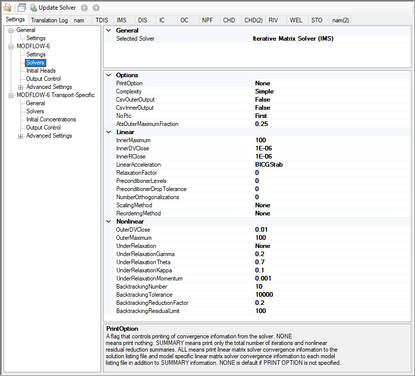
General Solution Options

The following settings are optional in the IMS package:

·    PrintOption: An optional keyword setting that determines the print level of the solver in the listing file:
                o    Summary means print only the total number of iterations and nonlinear residual reduction summaries.
                o    All means print linear matrix solver convergence information to the solution listing file and model specific linear matrix solver convergence information to each model listing file in addition to Summary information.
                o    None means that no solver information will be printed. This is the default option.
·    Complexity: is an optional keyword that defines default non-linear and linear solver parameters.

                o    Simple indicates that default solver input values will be defined that work well for nearly linear models. This option is generally suitable for models that do not include nonlinear stress packages and models that are either confined or consist of a single unconfined layer that is thick enough to contain the water table within a single layer.
                o    Moderate: indicates that default solver input values will be defined that work well for moderately nonlinear models. This option is generally suited for models that include nonlinear stress packages and models that consist of one or more unconfined layers. The Moderate option should be used when the Simple option does not result in successful convergence.
                o    Complex: indicates that default solver input values will be defined that work well for highly nonlinear models. This option is generally suited for models that include nonlinear stress packages and models that consist of one or more unconfined layers representing complex geology and surface-water/groundwater interaction. The complex option should be used when the moderate option does not result in successful convergence.
                o    Custom: indicates that custom values will be defined for the linear and non-linear solvers.

If the Simple, Moderate, or Complex options are selected, then only the items in the linear and non-linear solver sections below marked with * will be translated. All other options will use the defaults below:

·    CsvOuterOutput: if this option is set to yes, then outer iteration convergence information will be written to a comma separated values file in the GWF subfolder. This option is off by default. Information written to this file includes maximum dependent-variable (for example, head or concentration) change convergence information at the end of each outer iteration for each time step.
·    CsvInnerOutput: if this option is set to yes, then inner iteration convergence information will be written to a comma separated values file in the GWF subfolder. This option is off by default. Information written to this file includes maximum dependent-variable (for example, head or concentration) change and maximum residual convergence information for the solution and each model (if the solution includes more than one model) and linear acceleration information for each inner iteration.
·    NoPTC: is a settings that is used to control the pseudo-transient continuation (PTC) options for steady state periods for models using the Newton-Raphson formulation
(which is controlled by in NAM file settings):
o    None: PTC will not be used in solution
o    First: PTC will be activated for the first stress period
o    All: PTC will be deactivated for all stress periods

For many problems, PTC can significantly improve convergence behavior for steady-state simulations, and for this reason it is active by default. In some cases; however, PTC can worsen the convergence behavior, especially when the initial conditions are similar to the solution. When the initial conditions are similar to (or exactly the same as) the solution and convergence is slow, then the NO_PTC FIRST option should be used to deactivate PTC for the first stress period. The NO_PTC ALL option should also be used in order to compare convergence behavior with other MODFLOW versions, as PTC is only available in MODFLOW 6.

AtsOuterMaximumFraction: real value defining the fraction of the maximum allowable outer iterations used with the Adaptive Time Step (ATS) capability if it is active. If this value is set to zero by the user, then this solution will have no effect on ATS behavior. This value must be greater than or equal to zero and less than or equal to 0.5 or the program will terminate with an error. If it is not specified by the user, then it is assigned a default value of one third. When the number of outer iterations for this solution is less than the product of this value and the maximum allowable outer iterations, then ATS will increase the time step length by a factor of DTADJ in the ATS input file. When the number of outer iterations for this solution is greater than the maximum allowable outer iterations minus the product of this value and the maximum allowable outer iterations, then the ATS (if active) will decrease the time step length by a factor of 1 / DTADJ.

Non-Linear Solver Options

The following settings are available for the Non-linear solver:

·    OUTER_DVCLOSE: real value defining the dependent-variable (for example, head or concentration) change criterion for convergence of the outer (nonlinear) iterations, in units of the dependent-variable (for example, length for head or mass per length cubed for concentrations). When the maximum absolute value of the dependent-variable change at all nodes during an iteration is less than or equal to OUTER_DVCLOSE, iteration stops.
·    OUTER_MAXIMUM: integer value defining the maximum number of outer (nonlinear) iterations. For a linear problem OUTER_MAXIMUM should be 1.
·    UNDER_RELAXATION: an optional keyword that defines the nonlinear under-relaxation schemes used. Under-relaxation is also known as dampening, and is used to reduce the size of the calculated dependent variable before proceeding to the next outer iteration. Under-relaxation can be an effective tool for highly nonlinear models when there are large and often counteracting changes in the calculated dependent variable between successive outer iterations. By default under-relaxation is not used.
o    NONE [Default] - under-relaxation is not used
o    SIMPLE - Simple under-relaxation scheme with a fixed relaxation factor (under relaxation gamma (see below)) is used.
o    COOLEY - Cooley under-relaxation scheme is used.
o    DBD - delta-bar-delta (DBD) under-relaxation is used.

Note that the under-relaxation schemes are often used in conjunction with problems that use the Newton-Raphson formulation (which is controlled by in NAM file settings); however, experience has indicated that they also work well for non-Newton problems, such as those with the wet/dry options of MODFLOW 6.

·    UNDER_RELAXATION_GAMMA: a real value defining either the relaxation factor for the simple complexity scheme or the history or memory term factor of the Cooley and delta-bar-delta algorithms. For the simple scheme, a value of one indicates that there is no under-relaxation and the full head (or concentration) change is applied. This value can be gradually reduced from one as a way to improve convergence; for well behaved problems, using a value less than one can increase the number of outer iterations required for convergence and needlessly increase run times. Under relaxation gamma must be greater than zero for the simple scheme or the program will terminate with an error. For the Cooley and delta-bar-delta schemes, Under relaxation gamma is a memory term that can range between zero and one. When Under relaxation gamma is zero, only the most recent history (previous iteration value) is maintained. As Under relaxation gamma is increased, past history of iteration changes has greater influence on the memory term. The memory term is maintained as an exponential average of past changes. Retaining some past history can overcome granular behavior in the calculated function surface and therefore helps to overcome cyclic patterns of non-convergence. The value usually ranges from 0.1 to 0.3; a value of 0.2 works well for most problems. Under relaxation gamma is only used in the simulation if Under relaxation is not None.
·    UNDER_RELAXATION_THETA: a real value defining the reduction factor for the learning rate (underrelaxation term) of the delta-bar-delta algorithm. The value of under relaxation theta is between zero and one. If the change in the dependent-variable (for example, head or concentration) is of opposite sign to that of the previous iteration, the under-relaxation term is reduced by a factor of under relaxation theta. The value usually ranges from 0.3 to 0.9; a value of 0.7 works well for most problems. Under relaxation theta is only used in the simulation if under relaxation is DBD.
·    UNDER_RELAXATION_KAPPA: a real value defining the increment for the learning rate (under-relaxation term) of the delta-bar-delta algorithm. The value of under relaxation kappa is between zero and one. If the change in the dependent-variable (for example, head or concentration) is of the same sign to that of the previous iteration, the under-relaxation term is increased by an increment of under relaxation kappa. The value usually ranges from 0.03 to 0.3; a value of 0.1 works well for most problems. Under relaxation kappa is only used in the simulation if under relaxation is DBD.
·    UNDER_RELAXATION_MOMENTUM: a real value defining the fraction of past history changes that is added as a momentum term to the step change for a nonlinear iteration. The value of under relaxation momentum is between zero and one. A large momentum term should only be used when small learning rates are expected. Small amounts of the momentum term help convergence. The value usually ranges from 0.0001 to 0.1; a value of 0.001 works well for most problems. Under relaxation momentum is only used in the simulation if under relaxation is DBD.
·    BACKTRACKING_NUMBER: an integer value defining the maximum number of backtracking iterations allowed for residual reduction computations. If backtracking number = 0 then the backtracking iterations are omitted. The value usually ranges from 2 to 20; a value of 10 works well for most problems.

·    BACKTRACKING_TOLERANCE: a real value defining the tolerance for residual change that is allowed for residual reduction computations. The backtracking tolerance value should not be less than one to avoid getting stuck in local minima. A large value serves to check for extreme residual increases, while a low value serves to control step size more severely. The value usually ranges from 1.0 to 106; a value of 104 works well for most problems but lower values like 1.1 may be required for harder problems. Backtracking tolerance is only used in the simulation if backtracking number is greater than zero.
·    BACKTRACKING_REDUCTION_FACTOR: real value defining the reduction in step size used for residual reduction computations. The value of  is between zero and one. The value usually ranges from 0.1 to 0.3; a value of 0.2 works well for most problems. Backtracking reduction factor is only used in the simulation if backtracking number is greater than zero.
·    BACKTRACKING_RESIDUAL_LIMIT: a real value defining the limit to which the residual is reduced with backtracking. If the residual is smaller than backtracking residual limit, then further backtracking is not performed. A value of 100 is suitable for large problems and residual reduction to smaller values may only slow down computations. Backtracking residual limit is used in the simulation if backtracking number is greater than zero.

Linear Solver Options

The following settings are available for the Linear solver:

·    INNER_MAXIMUM: an integer value defining the maximum number of inner (linear) iterations. The number typically depends on the characteristics of the matrix solution scheme being used. For nonlinear problems, inner maximum usually ranges from 60 to 600; a value of 100 will be sufficient for most linear problems.
·    INNER_DVCLOSE: a real value defining the dependent-variable (for example, head or concentration) change criterion for convergence of the inner (linear) iterations, in units of the dependent-variable (for example, length for head or mass per length cubed for concentration). When the maximum absolute value of the dependent-variable change at all nodes during an iteration is less than or equal to inner dvclose , the matrix solver assumes convergence. Commonly, inner_dvclose is set equal to or an order of magnitude less than the outer_dvclose value specified for the non-linear block.
·    INNER_RCLOSE: a real value that defines the flow residual tolerance for convergence of the IMS linear solver and specific flow residual criteria used. This value represents the maximum allowable residual at any single node. Value is in units of length cubed per time, and must be consistent with MODFLOW-6 length and time units. Usually a value of 0.1 is sufficient for the flow-residual criteria when meters and seconds are the defined MODFLOW-6 length and time.

·    RCLOSE_OPTION: an optional keyword that defines the specific flow residual criterion used.
o    STRICT: an optional keyword that is used to specify that inner rclose represents a infinity-Norm (absolute convergence criteria) and that the dependent-variable (for example, head or concentration) and flow convergence criteria must be met on the first inner iteration (this criteria is equivalent to the criteria used by the MODFLOW-2005 PCG package (Hill, 1990)).
o    L2NORM_RCLOSE : an optional keyword that is used to specify that inner rclose represents a L-2 Norm closure criteria instead of a infinity-Norm (absolute convergence criteria). When L2norm rclose is specified, a reasonable initial inner rclose value is 0.1 times the number of active cells when meters and seconds are the defined MODFLOW-6 length and time.
o    RELATIVE_RCLOSE : an optional keyword that is used to specify that inner rclose represents a relative L-2 Norm reduction closure criteria instead of a infinity-Norm (absolute convergence criteria). When relative rclose is specified, a reasonable initial inner rclose value is 1.0×10- 4 and convergence is achieved for a given inner (linear) iteration when inner dvclose and the current L-2 Norm is the product of the relative_rclose and the initial L-2 Norm for the current inner (linear) iteration. If rclose option is not specified, an absolute residual (infinity-norm) criterion is used.
·    LINEAR ACCELERATION: a keyword that defines the linear acceleration method used by the default IMS linear solvers.
o    CG - preconditioned conjugate gradient method.
o    BICGSTAB - preconditioned bi-conjugate gradient stabilized method.
·    RELAXATION_FACTOR: an optional real value that defines the relaxation factor used by the incomplete LU factorization preconditioners (MILU(0) and MILUT).
Relaxation_factor is unitless and should be greater than or equal to 0.0 and less than or equal to 1.0. Relaxation factor values of about 1.0 are commonly used, and experience suggests that convergence can be optimized in some cases with relax values of 0.97. A Relaxation factor value of 0.0 will result in either ILU(0) or ILUT preconditioning (depending on the value specified for preconditioner levels and/or
preconditioner drop tolerance ). By default, relaxation factor is zero.
·    PRECONDITIONER_LEVELS: an optional integer value defining the level of fill for ILU decomposition used in the ILUT and MILUT preconditioners. Higher levels of fill provide more robustness but also require more memory. For optimal performance, it is suggested that a large level of fill be applied (7 or 8) with use of a drop tolerance. Specification of a preconditioner levels value greater than zero results in use of the ILUT preconditioner. By default, the number of preconditioner levels is zero and the zero-fill incomplete LU factorization preconditioners (ILU(0) and MILU(0)) are used.
·    PRECONDITIONER_DROP_TOLERANCE: a real value that defines the drop tolerance used to drop preconditioner terms based on the magnitude of matrix entries in the ILUT and MILUT preconditioners. A value of 10- 4 works well for most problems. By default, the preconditioner drop tolerance is zero and the zero-fill incomplete LU factorization preconditioners (ILU(0) and MILU(0)) are used.

·    NUMBER_ORTHOGONALIZATIONS: an integer value defining the interval used to explicitly recalculate the residual of the flow equation using the solver coefficient matrix, the latest dependentvariable (for example, head or concentration) estimates, and the right hand side. For problems that benefit from explicit recalculation of the residual, a number between 4 and 10 is appropriate. By default, the number of
orthogonalizations is zero.
·    SCALING_METHOD: an optional keyword that defines the matrix scaling approach used. By default, matrix scaling is not applied.
o    NONE [Default] - no matrix scaling applied.
o    DIAGONAL - symmetric matrix scaling using the POLCG preconditioner scaling method in Hill (1990).
o    L2NORM - symmetric matrix scaling using the L-2 Norm.
·    REODERING_METHOD: an optional keyword that defines the matrix reordering approach used. By default, matrix reordering is not applied.
o    NONE [Default] - original ordering.
o    RCM - reverse Cuthill McKee ordering.
o    MD - minimum degree ordering.

 

10.10.3.3 Initial Concentrations

In Visual MODFLOW Flex, the Initial Concentrations are typically defined at the Define Properties step in the workflow.  For more details, please see the section on setting Initial Concentrations. However, in some cases, it may be preferable to use alternate values from a previous model run. As such, the initial concentrations that will be translated for the simulation can be specified by species using the table shown below:

·    Id: The index of the species in the transport simulation as defined in the Modeling Objectives step.
·    Species Name: The name of the species
·    Option:
o    Specified [Default]:  will use the values that are defined for “Initial Concentrations” at the Define Properties step.

o    Previous_Run: requires you to select a .UCN file from a previous transport Run and specify the Time step to be used. The .UCN file must be based on the same grid type and number of cells in each applicable dimension (i.e. layer, row, and columns for a structured grid, and same number of layers and cells per layer for an unstructured grid).

Warning! Using Concentrations from Previous Run
The selected .UCN file cannot be the same as the .UCN file in the current translation directory. If you select Use .UCN from Previous Run option, you must choose a
.UCN file from another directory.

10.10.3.4 Output Control

The Output Control options set the information and frequency of information written and saved to the MODFLOW-6 output files (see following figure). 

By default, each MODFLOW-6 groundwater transport model simulation will produce several output files as described below.  The Output Control settings allow you to specify the stress period(s)/time step(s) for which model results of interest will be written to these output files. The Output Control Settings are provided in a tabular format:

·    Schedule:
o    End Time: the elapsed simulation time corresponding to the end of the specified stress period and time step
o    Stress Period: the stress period in the schedule
o    Time Step: the time step within the stress period
·    Save to Binary:
o    Concentration: simulated heads will be written to the binary heads file (.
\GWF\modelname.HDS) for active cells in the grid for selected End Times (Stress Period/Time Step)
o    Budget: mass budget terms will be written to the binary budget file (.
\GWF\modelname.BGT) for active cells and boundary conditions in the grid for selected End Times (Stress Period/Time Step).

 Please Note: for cell-by-cell values to be added to the budget file, the SAVE_FLOWS option must be enabled (set to "Yes") in the Advanced Settings for the NAM package. Similarly, for cell-to-boundary condition values to be added to the budget file, the SAVE_FLOWS option must be enabled in the Advanced Settings for each desired boundary condition (e.g. the SSM, CNC, and SRC packages). In Visual MODFLOW Flex, the SAVE_FLOWS option is enabled by default for all supported packages including the NAM file and supported boundary conditions.

Print to LST: information will be written to the listing file (.
\GWT\S###\modelname.LST), where S### is the index of each species:

o    Concentration: simulated concentrations will be written to the listing file for active cells in the grid for selected End Times (Stress Period/Time Step). Note that this option should be used sparingly, typically for model troubleshooting, particularly as this format can lead to overly large output files that are less efficient to work with than the binary file or related files that can be exported from Visual MODFLOW Flex.
o    Budget: net flow budget terms, expressed at a package level, for boundary conditions and internal storage will be written to the listing file for selected End Times (Stress Period/Time Step)

 Please Note: for cell-by-cell values to be added to the listing file, the PRINT_FLOWS option must be enabled (set to "Yes") in the Advanced Settings for the NAM package. Similarly, for cell-to-boundary condition values to be added to the budget file, the PRINT_FLOWS option must be enabled in the Advanced Settings for each desired boundary condition. In Visual MODFLOW Flex, the PRINT_FLOWS option is enabled by default for all supported packages including the NAM file and supported boundary conditions.

Saving Output Every Nth Time Step

For simulations with many stress periods and time steps, it can be very tedious to manually select the desired output time step intervals. The row of fields underneath the Output Control table are used to specify regular time step intervals for saving files during Each N-th step in each stress period. The first text box is where the N value is entered. To apply this value to the column, click the underlying checkbox. 
If a subsequent engine is included in the run formation (e.g. ZoneBudget) with the MODFLOW simulation, Visual MODFLOW Flex will save the flow terms for all time steps by default. 

10.10.3.5 Advanced Settings

Advanced translation settings are available for transport simulations to enable more advanced control of translation and package settings.  General and common settings are described in the section on the advanced settings for MODFLOW-6 groundwater flow (GWF) models, while package-specific settings are described below.

MODFLOW-6 - Transport Packages

Package-specific settings for MODFLOW-6 flow model packages are described below:

ADV Settings

The following settings are specific to the Advection (ADV) package:

·    Scheme - This setting allows you to select the solution technique for the transport:
o    Upstream [Default]: upstream finite difference
o    Central: central finite difference
o    TVD: Higher-order Total Variation Diminishing method

These methods are described in more detail, here and here.

CNC Settings

The following settings are specific to the Constant Concentration (CNC) package:

·    Duplicate CNC6 Cell Filter - When working with conceptual models, in some cases multiple constant concentration cells may be assigned to the same cell. When MODFLOW formulates the system of equations, it simply adds boundary conditions -for all other boundary conditions this is usually not a problem as these values still require a concentration solution for that cell; however adding the constant concentration values together typically does not produce the desired result.  Therefore, Visual MODFLOW Flex includes an optional filter to handle these cases on translation:
o    Minimum - the minimum specified concentration value for the current stress period in the cell(s) with multiple values will be assigned
o    Maximum - the maximum specified concentration value for the current stress period in the cell(s) with multiple values will be assigned
o    Average [Default] - the arithmetic mean of specified concentration values for the current stress period in the cell(s) with multiple values will be assigned
o    Sum - specified concentration values values for the current stress period in the cell(s) with multiple values will be added.

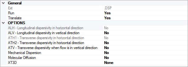
DSP Settings

The following settings are specific to the Dispersion (DSP) package and control how the Dispersion properties in the Define Properties workflow step will be translated:

·    ALH: a read-only setting for translating longitudinal dispersivity in the horizontal direction. If flow is strictly horizontal, then this is the longitudinal dispersivity that will be used. If flow is not strictly horizontal or strictly vertical, then the longitudinal dispersivity is a function of both ALH and ALV. If mechanical dispersion is included in the simulation (i.e. the Mechanical Dispersion setting is set to yes) then this settings is set to yes, otherwise, it is set to no.
·    ALV: a setting for translating longitudinal dispersivity in the vertical direction. If flow is strictly vertical, then this is the longitudinal dispersivity that will be used. If flow is not strictly vertical, then the longitudinal dispersivity is a function of both ALH and ALV. If this option is set to no and mechanical dispersion is represented, then the ALV values in the dispersion array is not translated and assumed to equal ALH by MODFLOW-6.
·    ATH1: a read-only setting for translating the transverse dispersivity in horizontal direction. This is the transverse dispersivity value for the second ellipsoid axis. If flow is strictly horizontal and directed in the x direction (along a row for a regular grid), then this value controls spreading in the y-direction. If mechanical dispersion is included in the simulation (i.e. the Mechanical Dispersion setting is set to yes) then this settings is set to yes, otherwise, it is set to no.
·    ATH2: a setting for translating the transverse dispersivity in horizontal direction. This is the transverse dispersivity value for the third ellipsoid axis. If flow is strictly horizontal and directed in the x direction (along a row for a regular grid), then this value controls spreading in the z-direction. If this option is set to no and mechanical dispersion is represented, then this array is not translated and assumed to equal ATH1 by MODFLOW-6.
·    ATV: a setting for translating the transverse dispersivity when flow is in vertical direction. If flow is strictly vertical and directed in the z-direction, then this value controls spreading in the x and y directions. If this option is set to no and mechanical dispersion is represented, then this array is not translated and assumed to equal ATH2 (or ATH1) by MODFLOW-6.

·    Mechanical Dispersion: a setting for translating the dispersivity terms (ALH, ALV, ATH1, ATH2, ATV). If set to yes, then ALH and ATH1 will values will be translated and the other dispersivity terms (ALV, ATH2, and ATV) will be translated based on their settings; otherwise, none of these terms will be included and mechanical dispersion terms will be omitted from the solution.
·    Molecular Diffusion: a setting for translating the diffusion term. If set to yes, then the molecular diffusion term will be included in the simulation.
·    XT3D: a setting for (de)activating the XT3D method and has the following options:
o    None [Default] : the XT3D formulation will not be used in the solution. This method is generally faster and less accurate. This option may provide a fast and accurate solution under some circumstances, such as when flow aligns with the model grid, there is no mechanical dispersion, or when the longitudinal and transverse dispersivities are equal. This option may also be used to assess the computational demand of the XT3D approach by noting the run time differences with and without this option on.
o    RHS : the XT3D formulation will only add dispersion terms to the right-hand side terms in the system of equations for the transport solution. This option uses less memory, but may require more iterations than the full XT3D formulation available by using the Coefficients option.
o    Coefficients: the full XT3D formulation will used and dispersion terms will be added to the coefficient matrix in the system of equations for the transport solution. This option uses the most memory and may be computationally expensive; however, this option may be required to accurately represent dispersion.

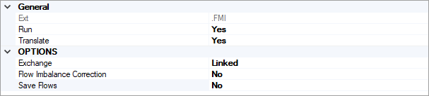
FMI Settings

The following settings are specific to the Flow Model Interface (FMI) package and control whether and how the Groundwater Flow (GWF) and Groundwater Transport (GWT) models will be linked:

·    Exchange: TBD
·    Flow Imbalance Correction: TBD
·    Save Flows: TBD

 Please Note: the FMI package and GWT6 (Exchange) package are mutually exclusive. 

IMST Settings

The following settings are specific to the Iterative Model Solution (IMS) package for Transport models (IMST):

·    UseSpeciesSpecificClosures: is a setting that controls whether or not the Species-Specific ClosureCriteria (see below) will be used. This option is set to no by default.
·    ClosureCriteria: Is a collection of species-specific settings that allows you to set independent solver closure criteria (i.e. INNER_DVCLOSE, INNER_RCLOSE, OUTER_DVCLOSE) for each species. This may be useful if the concentrations of the species are expected to vary over several orders of magnitude. To access the desired collection, click in the (Collection) cell and then click the  button. You can select more than one layer simultaneously using the mouse pointer and the [SHIFT] and
[CTRL] keys and define the criteria simultaneously for the selected layer(s).

IST Settings

The settings described below are specific to the Immobile Storage and Transfer (IST) package and will only be used if the Transport Modeling Objectives include either, the Dual Domain With Complex Sorption, the Triple Domain with Complex Sorption, or the Quadruple Domain with Complex Sorption Retardation Models.

The following settings are available for the active immobile domain(s) in the Immobile Storage and Transfer package:

·    Immobile1: is a collection of settings for the first immobile domain
·    Immobile2: is a collection of settings for the second immobile domain
·    Immobile3: is a collection of settings for the third immobile domain

Each one of these collections of settings can be accessed by clicking in the desired
(Collection) cell and clicking the  button, which will open the IST Immobile Domain Settings window with the following settings described below. You can select more than one layer simultaneously using the mouse pointer and the [SHIFT] and [CTRL] keys and define the criteria simultaneously for the selected layer(s).