韩松硬件加速2020最新综述：Model Compression and Hardware Acceleration for Neural Networks全文（中英文对照）连载中...

最新推荐文章于 2023-05-24 08:50:39 发布

robot.zhoy

最新推荐文章于 2023-05-24 08:50:39 发布

阅读量2k

点赞数 4

分类专栏： FPGA神经网络加速器文章标签：神经网络

本文链接：https://blog.csdn.net/weixin_44600457/article/details/113787883

版权

FPGA神经网络加速器专栏收录该内容

3 篇文章 3 订阅

订阅专栏

4 Neural Network acceleration: hardware

In this section, we introduce the hardware implementation of neural networks, from general-purpose processors to vanilla accelerators with sole hardware optimization and modern accelerators with algorithm-hardware codesign. Before presenting the details, we first explain the computation pattern of neural networks because it is the basis of the latter hardware design. Fig. 21 illustrates two typical workloads in running neural networks, that is, the Conv layer and the FC layer. The former features Conv operations while the latter features matrix–vector multiplications (MVMs). In the Conv operation, there is huge data reusability including both activations and weights; by contrast, the data cannot be reused in the MVM operation if without the batching technique. In fact, the computation of one sliding window in the Conv operation is equivalent to an MVM operation.

在本节中，我们将介绍神经网络的硬件实现，从通用处理器到具有单一硬件优化的普通加速器，以及具有算法-硬件协同设计的现代加速器。在详细介绍之前，我们首先说明神经网络的计算模式，因为它是后一种硬件设计的基础。图21为运行神经网络的两种典型工作方式，即Conv层和FC层。前者的特点是卷积运算，后者的特点是矩阵向量乘法(MVM)。在Conv操作中，存在大量的数据重用性，包括激活和权重;相比之下，如果没有批处理技术，数据就不能在MVM操作中重用。实际上，Conv操作中一个滑动窗口的计算相当于一个MVM操作。

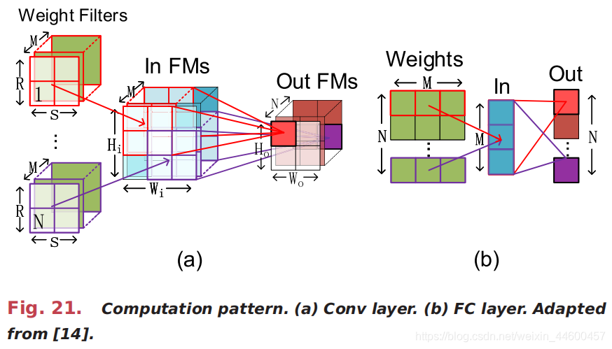
A. Why Domain-Specific Accelerator for Neural Networks?

Besides innovative algorithms, increasing data resources, and easy-to-use programming tools, the rapid development of neural networks also heavily relies on the computing capability of the hardware. The general-purpose processors such as GPUs act as the mainstay in the deep learning era, especially on the cloud side. GPUs keep an ongoing pursuit of high throughput, whereas they pay the cost of huge resource overhead and energy consumption.

除了创新的算法、增加的数据资源和易于使用的编程工具外，神经网络的快速发展还严重依赖于硬件的计算能力。 GPU等通用处理器在深度学习时代起着中流砥柱的作用，特别是在云计算方面。 GPU一直追求高吞吐量，然而他们付出的代价是巨大的资源开销和能源消耗。

For the edge applications, the budget on resource and energy is usually very limited. How to minimize the latency, energy, and area has become an inevitable design concern. Although the use of on-GPU compression such as [201], [233], [250], and [251] can improve the performance, there is still a big gap far from our expectation due to the redundant design of general-purpose processors for flexible programmability and general applicability. This motivates the study of specialized accelerators tailored for neural networks. By sacrificing the flexibility to some extent, these accelerators focus on the specific pattern of neural networks to achieve satisfactory performance through the optimization of processing architecture, memory hierarchy, and dataflow mapping. Note that most neural network accelerators are intended for the inference phase and the CNN models due to their wide applications on the edge side. Although we can find a few ones for the training phase [252]–[254], RNN models [255] or both CNNs and RNNs [256]–[258], they are still not the mainstream. Therefore, the default neural network accelerators in this article indicate the CNN inference scenario unless otherwise specified. Due to the limited space, we just review the recent accelerators that can support large-scale neural networks and ignore the early ones [259], [260].

对于边缘应用，资源和能源的预算通常非常有限。如何使延迟、能量和面积最小化成为设计中不可避免的问题。虽然使用针对GPU的压缩技术[201]、[233]、[250]、[251]可以提高性能，但由于通用处理器的冗余设计，使得距具有灵活的可编程性和通用性，仍然有很大的差距，与我们的预期相距甚远。这激发了专门为神经网络设计的加速器的研究。这些加速器在一定程度上牺牲了灵活性，专注于特定的神经网络模式，通过优化处理体系结构、内存层次结构和数据流映射来实现令人满意的性能。请注意，大多数神经网络加速器用于推理阶段和CNN模型，因为它们在边缘方面的应用非常广泛。虽然我们可以找到一些用于训练阶段[252]-[254]、RNN模型[255]或CNN和RNN[256] -[258]的模型，但它们仍不是主流。因此，除非另有说明，本文中默认的神经网络加速器表示CNN推理场景。由于篇幅有限，我们只回顾了最近支持大规模神经网络的加速器，而忽略了早期的加速器[259]，[260]。

B. Sole Hardware Optimization

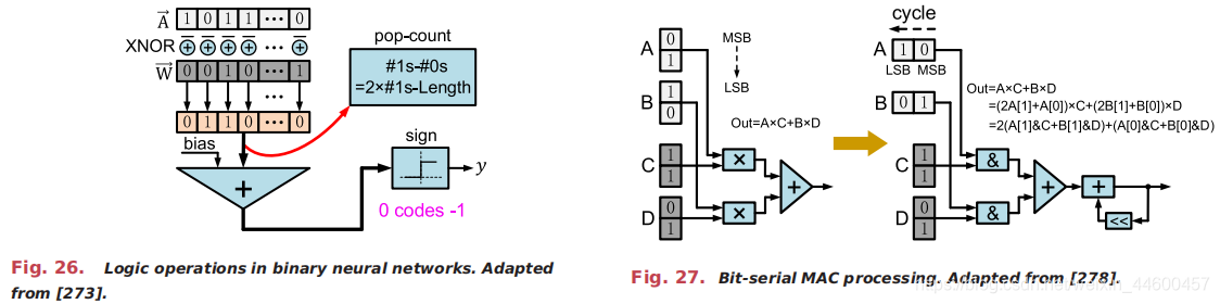
1) Parallel Compute Units and Orchestrated Memory Hierarchy: Usually, neural network accelerators make efforts in two aspects: enhancing the compute parallelism and optimizing the memory hierarchy. For example, DaDianNao [8] distributed weight memory into multiple tiles for the better locality. The MAC operations are performed in parallel by these tiles and the intermediate activations of different tiles are exchanged through a central memory. By contrast, in other neural network accelerators (e.g., Eyeriss [261], TPU [9], and Thinker [257]), the architecture often has an array of processing elements (PEs) with a small local buffer for each and a global buffer to hide the off-chip DRAM access latency, as shown in Fig. 22. Double buffering technique can be used in the global buffer to prefetch data before layer computation [257].
1) 并行计算单元和灵活组合内存层次结构:通常，神经网络加速器从两个方面展开:增强计算的并行性和优化内存层次。例如，DaDianNao[8]将权重内存分配到多个块中，以获得更好的性能。MAC操作是由这些块和不同的中间激活并行执行的拼接通过一个中央存储器交换。相比之下，在其他神经网络加速器(如Eyeriss[261]、TPU[9]和Thinker[257])中，该体系结构通常有一组处理元素(PE)，每个处理元素都有一个小的本地缓冲区，还有一个全局缓冲区来隐藏片外DRAM访问延迟，如图22所示。在全局缓冲区中可以使用双缓冲技术，在层计算之前预取数据[257]。

The PE array features a dataflow processing fashion with an orchestrated network-on-chip (NoC) enabling direct message passing between PEs. Three types of data, input activation, weight, and partial sum (psum) of output activation, flow through the PE array when performing a Conv or MVM operation, which increases the data reuse thus decreasing the requirement for memory bandwidth. Furthermore, the dataflow pattern can be variable in a different design. We use Fig. 23 to briefly explain it. As depicted in Fig. 23(a), the output psum is stationary in each PE, and the input activations and weights propagate across PEs along the row and column directions, respectively. In this way, the inputs and weights can be reused by multiple PEs, which can reduce the memory access. Besides the output stationary dataflow [257], we can also see architectures with input stationary dataflow [262] or weight stationary dataflow [9], as shown in Fig. 23(b) and (c). Eyeriss [261] uses another dataflow called row stationary dataflow that is illustrated in Fig. 23(d). Specifically, each PE performs the Conv operation between one weight row and one input row, and the PEs in the same column generates one output row. The weights and psums propagate across PEs along the row and column directions, respectively, whereas the input activations propagate along the diagonal direction that is different from other dataflow solutions mentioned above.

PE阵列采用了一种数据流处理方式，通过设计的片上网络(NoC)实现PE之间的直接消息传递。当执行Conv或MVM操作时，PE阵列中有三种类型的数据:输入激活、权重和输出激活的部分和(psum)，这增加了数据的重用性，从而降低了对内存带宽的要求。此外，数据流模式在不同的设计中可以是可变的。我们用图23来简单解释一下。如图23(a)所示，输出psum在每个PE中是平稳的，而输入激活和权值分别沿着行方向和列方向在PE中传播。这样，输入和权值可以被多个PE重用，从而减少了内存访问。除了输出固定数据流[257]，我们也可以看到在图23(b)和(c)中有输入平稳数据流[262]和权重平稳数据流[9]的架构。Eyeriss[261]使用了另一种称为行平稳数据流的数据流，如图23(d)所示。具体来说，每个PE在一个权重行和一个输入行之间执行Conv操作，同一列的PE生成一个输出行。权重和pme分别沿行方向和列方向在PE之间传播，而输入激活则沿不同于上述其他数据流解决方案的对角线方向传播。

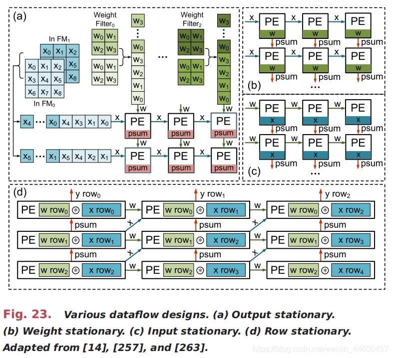
Combining the weight distribution [8] with the inter-PE data passing [9], [257], Tianjic [264], [265] and Simba [266], [267] adopt a scalable many-core/many-chip architecture where all cores (i.e., PEs) work in a decentralized manner without the global off-chip memory. Compared with the above accelerators, this emerging architecture is more spatial, as presented in Fig. 24. The weights are preloaded into each PE and remain stationary during the entire inference, and the activations propagate across intrachip and interchip cores.

将权重分配[8]与PE间数据传递[9]、[257]、Tianjic[264]、[265]和Simba[266]相结合，采用可扩展的多核/多芯片体系结构，其中所有核(即PE)都以分散的方式工作，而不需要全局片外存储器。与上述加速器相比，这种新兴的体系结构更具空间性，如图所示 24. 权重被预加载到每个PE中，并在整个推理过程中保持不变，并且激活在芯片内和芯片间传输。

2) Processing-in-Memory (PIM) Architecture: In conventional digital neural network accelerators, an MVM operation is split into many MAC operations to perform cycle by cycle. To improve the efficiency of performing MVM the PIM architecture based on emerging nonvolatile memory (eNVM) technologies has been widely studied. Taking memristor (e.g., RRAM [268], PCRAM [252]) as an example, the MVM can be performed in the analog domain. Each column of the crossbar obeys $I_{j}$ = $\Sigma _{i}V_{i}G_{ij}$ , where $V_{i}$ is the input voltage of the ith row, $I_{j}$ is the output current of the j th column, and $G_{ij}$ is the memristor device conductance at the (i,j)th crosspoint. The weights are prestored as G, and the input and output activations correspond to V and I, respectively. The entire MVM can be processed in the analog domain with only one cycle, which is ultrafast. Nevertheless, ADCs (ADCs and DACs) are usually needed, which causes extra overhead. For the current to voltage (I2V) converters, they can be implemented either explicitly [258], [268] or implicitly [269] in different designs. The complete architecture is similar to the spatial architectures in [264]–[267] (see Fig. 24), where each MVM engine is a weight-stationary PE and a communication infrastructure helps the activation passing between PEs. Besides the MVM operation, some other operations such as scalar and vector operations should be additionally supported by PEs since they are necessary for some neural network models such as RNNs but cannot be handled by the memristor array efficiently [258]. Besides eNVM devices, traditional memories such as SRAM [270],DRAM [271], and Flash [272] can also be modified to support the PIM-fashion processing of neural networks. However, only small-scale prototype chips have been taped out due to the difficulty in fabrication, therefore they are not widely used in industry although they are very hot in academia.

2)内存中处理(PIM)体系结构:在传统的数字神经网络加速器中，一个MVM操作被分割成多个MAC操作，一个周期一个周期地执行。为了提高MVM的执行效率，基于新兴非易失性内存(eNVM)技术的PIM体系结构得到了广泛的研究。以忆阻器(如RRAM [268]， PCRAM[252])为例，MVM可以在模拟域进行。交叉开关的每一列都服从 $I_{j}$ = $\Sigma _{i}V_{i}G_{ij}$ ，其中 $V_{i}$ 为第i行输入电压， $I_{j}$ 为第j列输出电流， $G_{ij}$ 为第(i,j)个交点处的忆阻器件电导。权值预存储为G，输入和输出激活分别对应V和I。整个MVM可以在模拟域内处理，只需一个周期，速度非常快。然而，通常需要ADC (ADC和DAC)，这造成了额外的开销。对于电流-电压(I2V)转换器，它们可以在不同的设计中显式实现[258]、[268]或隐式实现[269]。完整的架构类似于[264]-[267]中的空间架构(见图24)，其中每个MVM引擎是一个权重固定的PE，通信基础设施帮助激活PE之间的传递.除了MVM操作，一些其他的操作，如标量和向量操作，PEs需要额外支持，因为这些操作对于一些神经网络模型(如RNNs)是必需的，但忆阻器阵列不能有效地处理[258]。除了eNVM设备外，传统的存储器如SRAM[270]、DRAM[271]、Flash[272]也可以被修改以支持神经网络的PIM方式处理。然而，由于制造的困难，目前只有小规模的芯片原型，因此尽管在学术界非常热门，但在工业上还没有广泛的应用。

C. Algorithm and Hardware Codesign

The above optimizations from the sole hardware side gradually meet the performance wall when the parallelism and data reuse are exhausted. Therefore, researchers start to seek help from both algorithm and hardware sides, termed algorithm-hardware codesign. Since then, various compression techniques for neural networks mentioned earlier in this article are widely exploited in the design of

modern accelerators.

当并行性和数据重用耗尽时，上述单一硬件侧的优化逐渐达到性能瓶颈。因此，研究者开始从算法和硬件两方面寻求帮助，即算法-硬件协同设计。自此，本文前面提到的各种神经网络压缩技术在现代加速器设计中得到了广泛的应用。

1) Transformation Into Compact Model: Compact models are able to shrink the model size, and they do not change the dense execution pattern and data precision as usual neural networks. Although they can directly run on most platforms, including both general-purpose processors and specialized accelerators, their compact connections/operations and variable data paths might degrade the hardware utilization. Eyeriss V2 [10] addresses this issue by codesigning flflexible tiling/mapping schemes and an effificient NoC infrastructure with both high bandwidth and high data reuse. In addition, some compressed networks produced by other approaches can also be transformed into compact models. For example, the quantized networks can be viewed as dense models with shorter bit-width [179]; structurally pruned networks(e.g., vector-wise in RNNs and FM-wise in CNNs) [204],[205], [232], [234] or decomposed networks [139] can be reassembled into smaller dense models to speed up

the running.

1) 向紧凑模型的转换: 紧凑模型能够缩小模型的大小，并且不像通常的神经网络那样改变密集的执行模式和数据精度。尽管它们可以直接在大多数平台上运行，包括通用处理器和专用加速器，但它们紧凑的连接/操作和可变的数据路径可能会降低硬件利用率。Eyeriss V2[10]通过共同设计灵活的平铺/映射方案和高效的高带宽和高数据重用的NoC基础设施解决这个问题。此外，其他方法产生的一些压缩网络也可以转化为紧凑的模型。例如，量化后的网络可以看作是位宽较短的密集模型[179];(如结构修剪网络。[204]、[205]、[232]、[234]或分解后的网络[139]可以重新组装成更小的密集模型，以提高速度的运行。

2) Tensorized Processing Engine: As mentioned above, most decomposed networks can be described as dense matrix operations with a smaller size, which are still suitable for running on general-purpose processors [139]. However, it is worth noting that for the tensor decomposition cases [4], [121], some abnormal operations are induced (e.g., dimension reshape of tensor cores and intermediate results), needing additional support if higher effificiency is expected. Recently, TIE [11] accelerates the TT decomposed neural networks, where the reshape is implemented by partitioning the working SRAM into multiple groups with a well-designed data selection mechanism. Fig. 25 illustrates a detailed example of TT-decomposed MVM to help understanding. The original dimension information is W ∈ $\mathbb{R}^{4\times 18}$ , X ∈ $\mathbb{R}^{18\times 1}$ , and Y ∈ $\mathbb{R}^{4\times 1}$ . Using the TT decomposition, they are tensorized with dimensions of X ∈ $\mathbb{R}^{2\times3\times3}$ , and Y ∈ $\mathbb{R}^{2\times1\times2}$ , G 1 ∈ $\mathbb{R}^{2\times(1\times3)\times2}$ , G 2 ∈ $\mathbb{R}^{1\times(3\times3)\times3}$ , G 3 ∈ $\mathbb{R}^{2\times(3\times1)\times3}$ , where W = reshape ( $G_{1}\times ^{1}G_{2}\times^{1}\times G_{3}$ ) [here the symbol G is equivalent to G in (21)]. Then the MVM is transformed into tensor contractions of Y = ( $G_{1}\times ^{2}(G_{2}\times^{2}\times( G_{3}\times^{1}X))$ , from the right side to the left side corresponding to the step 1 – 3 in Fig. 25. The tensor contractions are essentially implemented by fifirst matricizing the tensors into matrices and performing matrix–matrix multiplication in a PE array. After each contraction step, the intermediate output Y should be reshaped to Y for the computation of the next step. To realize the reshape effificiently, TIE provides an SRAM partition scheme. The memory consists of multiple groups and multiple chunks in each group. At each cycle, it reads a fraction of required data from different memory chunks and then assembles them into a new row that is expected in the reshaped format. For each chunk, the access addresses are continuous with high effificiency. In this way, the reshape operation is completed virtually, which does not consume any extra overhead.

2) 张量处理机: 如上所述，大多数分解网络可以描述为密集矩阵操作，但规模较小，仍然适合在通用处理器上运行[139]。但是，值得注意的是，对于张量分解案例[4][121]，会导致一些异常操作(如张量核的维数重构和中间结果)，如果想要获得更高的效率，需要额外的支持。最近，TIE[11]加速了TT分解的神经网络，通过一个精心设计的数据选择机制将工作的SRAM分成多个组来实现重构。图25给出了TT分解MVM的详细示例，以帮助理解。原始维数信息是 W ∈ $\mathbb{R}^{4\times 18}$ , X ∈ $\mathbb{R}^{18\times 1}$ , and Y ∈ $\mathbb{R}^{4\times 1}$ 。通过TT分解，对 X ∈ $\mathbb{R}^{2\times3\times3}$ , and Y ∈ $\mathbb{R}^{2\times1\times2}$ , G 1 ∈ $\mathbb{R}^{2\times(1\times3)\times2}$ , G 2 ∈ $\mathbb{R}^{1\times(3\times3)\times3}$ , G 3 ∈ $\mathbb{R}^{2\times(3\times1)\times3}$ 的维数进行张量化，其中W = 重构 ( $G_{1}\times ^{1}G_{2}\times^{1}\times G_{3}$ )[这里符号G等价于在(21)中的G]。然后将MVM转换为 Y = ( $G_{1}\times ^{2}(G_{2}\times^{2}\times( G_{3}\times^{1}X))$ 的张量收缩，从右侧到左侧，对应图25中的步骤1 - 3。张量收缩本质上是首先将张量矩阵化为矩阵并在PE数组中执行矩阵-矩阵乘法来实现的。在每一个收缩步骤之后，中间输出Y应该被重构，以便计算下一步。为了有效地实现重构，TIE提出了SRAM的分区方案。内存由多个组和每个组中的多个块组成。在每个周期中，它从不同的内存块中读取所需数据的一部分，然后将它们组合到一个新的行中，该行将以重新格式化的格式出现。对于每个数据块，访问地址都是连续的，效率高。这样，整形操作是虚拟完成的，不会消耗任何额外的开销。

3) Quantized Architecture: With negligible accuracy loss, the required data precision is usually ≥ 8-bit fifixed point for CNN inference [8], [9]. Whereas, more aggressive low-bit quantization can be seen in the research community for the pursuit of ultrahigh execution performance with a certain degree of accuracy loss, which is the focus here. There are two categories of quantized neural network architecture: for fifixed bitwidth or for variable bitwidth.

3)量化架构: CNN推理[8]、[9]所需的数据精度通常≥8位浮点数，精度损失可以忽略。而在研究界，为了追求超高的执行性能，在一定程度的精度损失的情况下，可以看到更激进的低位量化方法，这是本文的重点。量化神经网络体系结构分为固定位宽和可变位宽两类。

For the cases with fifixed bitwidth, we can easily replace the high-precision multipliers and adders with identically lower-bit ones, and the overall architecture and dataflflow remain the same as conventional ones mentioned in Section IV-B. Here, we emphasize the extreme quantization with only binary/ternary data precision. If only the weights are binarized/ternarized, the costly MAC operations can be reduced to simpler accumulations [274]. If both the weights and activations are binarized/ternarized, the MAC operations can be implemented by quite simple XNOR and pop-count logic operations [273], [275]–[277], which is illustrated in Fig. 26. Compared to binarization, ternarized neural networks can further exploit the sparsity due to the extra zero values.

对于位宽固定的情况，我们可以很容易地将高精度乘法器和加法器替换为相同的低位乘法器和加法器，并且总体架构和数据流与第IV-B节中提到的常规乘法器和加法器保持一致。在这里，我们强调只有二进制/三元数据精度的极端量化。如果只将权值二值化/三值化，那么昂贵的MAC操作就可以减少为更简单的累加[274]。如果权重和激活都是二进制/三元化的，MAC操作可以通过相当简单的XNOR和pop-count逻辑运算来实现，如图26所示。与二值化相比，三值化的神经网络由于额外的零值可以进一步利用稀疏性。

For the cases with variable bitwidth, the motivation is that the required bitwidth probably varies across layers and models rather than always keeping uniform [176]. To this end, it is better to provide flflexible architectural support for variable bitwidth. Two ways are utilized in this context: bit-serial [12], [278] and bit-decomposed [279], which are depicted in Figs. 27 and 28, respectively. Different from the normal bit-parallel processing, the bitserial processing serially feeds one of the two operands bit by bit at each cycle. In this way, the MAC operations can be transformed into AND logic operations and shifted accu mulations. Because the single MAC operation now needs more cycles, the bit-serial processing usually uses more PEs to enhance the parallelism. Owing to the mutiplierless architecture, this causes only a little area overhead but achieving continuous bitwidth support. The performance gain linearly increases with the bitwidth reduction. The bit-decomposed scheme fuses multiple low-precision MACs with shifted accumulations to form a higher precision MAC. The fusion group size is confifigurable to support flflexible bitwidth. Compared to the bit-serial architecture, the bit-decomposed one can quantize both operands while paying the cost of discontinuity in the bitwidth distribution.

对于可变位宽的情况，其动机是所需的位宽可能会随着层和模型的不同而变化，而不是总是保持一致[176]。为此，最好为可变位宽提供灵活的架构支持。在这种情况下使用两种方式:位串行[12]，[278]和位分解[279]，分别见图27和图28。与普通的位并行处理不同的是，位串行处理在每个周期逐位串行地输入两个操作数中的一个。这样，MAC运算就可以转化为和逻辑运算和移位累加。由于单MAC操作现在需要更多的周期，位串行处理通常使用更多的PE来增强并行性。由于无乘数架构，这只会导致很少的区域开销，但可以实现连续的位宽支持。性能增益随位宽减小而线性增加。位分解方案将多个低精度MAC与移位累积融合，形成高精度MAC。融合组的大小是可配置的，以支持柔性位宽。与位串行结构相比，位分解的结构可以量化两个操作数，同时付出位宽分布不连续的代价。

In addition, the tradeoff between the model accuracy and the execution performance should be carefully considered. Su et al. [280] profifiled this tradeoff in inference via building a throughput estimation model. They conclude that on small-size data sets (e.g., MNIST or CIFAR10) INT2 or INT4 can reach a good tradeoff, while on large-size data sets (e.g., ImageNet) INT4 is the best choice. In HAQ [176], an RL-based AutoML approach is utilized to quantize neural networks considering both the accuracy loss and the latency/energy cost fed back from a simulated neural network accelerator.

此外，应该仔细考虑模型精度和执行性能之间的权衡。Su等人[280]通过建立一个 吞吐量估计模型在推理中描述了这种权衡。他们得出的结论是，在小型数据集(例如，MNIST或CIFAR10)上，INT2或INT4可以达到良好的折衷，而在大型数据集(例如，ImageNet)上，INT4是最佳选择。在HAQ[176]中，基于RL的AutoML方法被用来量化神经网络，考虑精度损失和从模拟神经网络加速器反馈的延迟/能量成本.

4) Sparse Architecture: In the family of sparse neural network accelerators, the exploitable sparse patterns include weight sparsity, input sparsity, output sparsity, and the combination of multiple patterns, which will be discussed one by one.

4)稀疏架构: 在稀疏神经网络加速器中，可利用的稀疏模式包括权值稀疏性、输入稀疏性、输出稀疏性以及多个模式的组合，我们将逐一讨论。

Early sparse accelerators leverage weight sparsity by naively skipping the MACs with zero weights. Fig. 29 gives an implementation example adapted from Cambricon-X [281]. The weights are stored in a sparse format with addressing indexes. Each PE accesses the required activations according to the weight index and then performs the residual MACs. In this way, the number of operations can

be reduced to a great extent, thus lowering the latency and energy. Nevertheless, the distribution of nonzero weights is usually very irregular, which causes large indexing overhead, PE imbalance, and memory access ineffificiency.

早期的稀疏加速器通过天真地跳过零权重的MAC来利用权重的稀疏性。图29给出了改编自Cambricon-X[281]的实现实例。权值以带有寻址索引的稀疏格式存储。每个PE根据权重索引访问需要的激活，然后执行剩余的MAC。这样，操作的数量就可以了被极大地减少，从而降低了延迟和能量。然而，非零权值的分布通常非常不规则，导致索引开销大，PE不平衡，内存访问效率低。

To this end, structured sparse patterns mentioned in Fig. 18 have been further exploited. For example, the block-wise weight sparsity is leveraged to optimize the running performance on general-purpose processors [13], [220], [234], and a more aggressive diagonal weight matrix is utilized in the accelerator design [282]. In these architectures, the required indexes can be greatly decreased, the number of MACs in each PE becomes more balanced, and the memory organization/access can be more effificient. Fig. 30 shows an example of exploiting vector-wise sparsity in a systolic array [263]. The nonzero weights on multiple columns (e.g., two adjacent columns in this example) are combined together by only remaining the absolutely largest element on each row (the rest are pruned).Actually, a greedy column combining and iterative training is used to guarantee accuracy. Each PE buffers the nonzero weights with a column index, and a multiplexer is additionally integrated to select the correct

input according to the weight column index.

为此，图18中提到的结构化稀疏模式得到了进一步的开发。例如，利用块加权稀疏来优化通用处理器[13]，[220]，[234]的运行性能，在加速器设计中使用了更激进的对角加权矩阵[282]。在这些体系结构中，所需的索引可以大大减少，每个PE中的MAC数量变得更加平衡，内存组织/访问可以更加高效。图30显示了在收缩阵列中利用矢量稀疏性的示例[263]。多列上的非零权重(例如，本例中相邻的两列)被组合在一起，只保留每行上绝对最大的元素(其余的被修剪)。实际上，为了保证准确性，采用了贪婪列组合和迭代训练的方法。每个PE用一个列索引缓冲非零权重，并且额外集成一个多路复用器来选择正确的权重按权重列索引输入。

robot.zhoy

关注

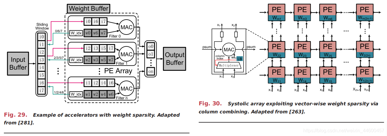
4
点赞
踩
13

收藏

觉得还不错? 一键收藏
0
评论
韩松硬件加速2020最新综述：Model Compression and Hardware Acceleration for Neural Networks全文（中英文对照）连载中...

@[TOC]## 4 Neural Network acceleration: hardwareIn this section, we introduce the hardware implementation of neural networks, from general-purpose processors to vanilla accelerators with sole hardware optimization and modern accelerators with algorithm
复制链接

扫一扫